Deep Transfer Learning on Small Dataset
The success of Convolutional Neural Network (ConvNet) application on image classification relies on two factors (1) having a lot of data (2) having a lot of computing power; where (1) having data seems to be a harder issue. Data acquisition is generally the major costs of any realistic project. But if we only can afford a small dataset, can we still use ConvNet effectively?
The Transfer Learning technique is using an existing ConvNet feature extraction and the associated trained network weights, transferring to be used in a different domain. The researches indicated the ConvNet exploits the hierarchical distributed representations. The lower layers of a ConvNet contain more generic features (e.g. edge detectors or color blob detectors) that should be useful to many tasks, but higher layers of the ConvNet becomes more specific to the details of the domain classes contained in the original dataset.
[2024/10/07] We can listen to this article as a Podcast Discussion, which is generated by Google’s Experimental NotebookLM. The AI hosts are both funny and insightful.
images/deep-transfer-learning-on-small-dataset/Podcast_Deep_Transfer_Learning.mp3
The Keras Blog on “Building powerful image classification models using very little data” by Francois Chollet is an inspirational article of how to overcome the small dataset problem, with transfer learning onto an existing ConvNet. Since modern ConvNets take 2-3 weeks to train across multiple GPUs on ImageNet (which contains 1.2 million images with 1000 categories), it is common to see people release their final ConvNet trained weight for the benefit of others who can use the networks for fine-tuning. For example, the Caffe library has a Model Zoo where people share their network weights. However, the higher layers weights may need to be fine-tuned. In the case of network using ImageNet dataset which contains many dogs and cats, a significant portion of the network weights may be devoted to features that are specific to differentiate between breeds of dogs in the higher layers, which are not as useful to a different domain. The transfer learning strategy must take into consideration.

Figure. VGG16 ConvNet Fine-Tuning Technique for adapting to different domain
A good transfer learning strategy is outlined as following steps:
- Freezing the lower ConvNet blocks (
blue) as fixed feature extractor. Take a ConvNet pretrained on ImageNet, remove the last fully-connected layers, then treat the rest of the ConvNet as a fixed feature extractor for the new dataset. In an VGG16 network, this would compute a 4096-D vector for every image that contains the activations of the hidden layer immediately before the classifier. These features are termed as CNN codes. - Training the new fully-connected layers (
green, aka. bottleneck layers). Extract the CNN codes for all images, train a linear classifier (e.g. Linear SVM or Softmax classifier) for the new dataset. - Fine-tuning the ConvNet. Replace and retrain the classifier on top of the ConvNet on the new dataset, but to also fine-tune the weights of the pretrained network by continuing the back-propagation to part of the higher layers (
yellow+green).
Transfer Learning Experiments
This section reports 3 experiments that applying the previous outlined transfer learning strategy. For each experiment, there is a specific question that we must learn.
- Kaggle’s Dogs vs Cats - to learn how to use the techniques.
- Oxford’s 102 Category Flower - to answer if large number of catergories can be adapted.
- UEC’s Food 100 - to answer if food/snack watching can be adapted.
Experiment Setup
The previous blog posts on Deep Style Transfer and Deep Dream have served to instruct how to setup on Windows 10. These experiments are setup using NVidia GTX 1070 GPU with CUDA 8.0 running on Windows 10. All softwares are written in Python using Keras configured to use Theano backend.
Due to the incompatibility of the latest CUDA 8.0 and the latest Keras version, the following step helps to downgrade Keras to 1.2.0 if needed.
Downgrade to Keras 1.2.0
In order to following the “image classification” blog’s code here, just downgrade to Keras 1.2.0 solved the running issue.
Find Keras version,
python -c "import keras; print keras.__version__"
If the reported Keras version is greater than 1.2.0, follow these steps to downgrade.
pip uninstall keras
pip install keras==1.2.0
Experiment 1: Dogs vs Cats Dataset
Following the article “Building powerful image classification models using very little data”, the two sets of pictures, which downloaded from Kaggle: 1000 cats and 1000 dogs (extracted from the original dataset which had 12,500 cats and 12,500 dogs, only the first 1000 images for each class is used). We also use 400 additional samples from each class as validation data, to evaluate the models.
Here are some sample images of the “Dog vs Cat” dataset. Some images are definitely challenging, for example, the animal is partially obscured or the scenery is not ideal.
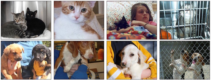
Figure. Dogs vs Cats dataset image samples
Each training epoch takes 20s on NVidia GTX 1070 GPU.
$ python classifier_from_little_data_script_3.py

Found 2000 images belonging to 2 classes.
Found 800 images belonging to 2 classes.
Epoch 1/50
2000/2000 [==============================] - 20s - loss: 0.4330 - acc: 0.8995 - val_loss: 0.3401 - val_acc: 0.8900
Epoch 2/50
2000/2000 [==============================] - 19s - loss: 0.2412 - acc: 0.9140 - val_loss: 0.3244 - val_acc: 0.9113
...
Epoch 49/50
2000/2000 [==============================] - 21s - loss: 0.0116 - acc: 0.9955 - val_loss: 0.4171 - val_acc: 0.9375
Epoch 50/50
2000/2000 [==============================] - 21s - loss: 0.0190 - acc: 0.9935 - val_loss: 0.3553 - val_acc: 0.9300
The fine-tuning process shows the accuracy is improving over the number of training epoch,
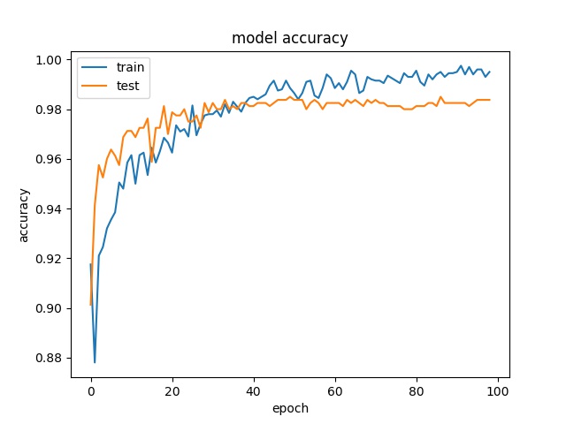
The overall validation accuracy is reaching 93%, which is pretty impressive. Thanks to the original VGG16 ImageNet network weights are having so many dogs and cats in the basic feature extractions. Even with a small dataset of 1000 dogs and 1000 cats picture, we could still achieve great accuracy.
Experiment 2: Oxford 102 Category Flower
Following the coding improvement by Alexander Lazarev’s Github code which make dataset setup and the number of classes setup more flexible, we are ready to see if ConvNet transfer learning strategy can be easily applied to a different domain on flowers. The Oxford 102 Category Flower Dataset is the flowers commonly appearing in the United Kingdom. Each class consists of between 40 to 258 images.
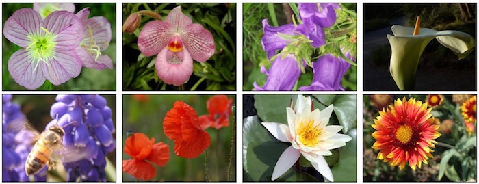
Figure. Oxford 102 Category Flower dataset image samples
Here is the list of the flower categories in the dataset, http://www.robots.ox.ac.uk/~vgg/data/flowers/102/categories.html
Notes on Windows 10:
model/vgg16.pyneeds to modify the NumPy array saving as ‘wb’ (write data with binary mode) and reading as ‘rb’ (read with binary mode).
Alex’s improved code can be used for any dataset, just follow the original files structure in data/sorted directory after running bootstrap.py. If you wish to store your dataset somewhere else, you can do it and run train.py with setting a path to dataset with a special parameter --data_dir==path/to/your/sorted/data.
Training process is fully automated and the best weights for the model will be saved.
Each epoch is taking 55-65s on a NVidia GTX 1070 GPU. It is a bigger dataset comparing with the previous Dogs vs Cats experiment. The log shows after the model is reloaded to do fine-tune.
$ python train.py --model=vgg16 --data_dir=flower/sorted
....
Weights for "fc1" are loaded
Weights for "fc2" are loaded
Weights for "predictions" are loaded
Found 6149 images belonging to 102 classes.
Found 1020 images belonging to 102 classes.
Epoch 1/300
6149/6149 [==============================] - 92s - loss: 11.5339 - acc: 0.4261 - val_loss: 7.1121 - val_acc: 0.4627
....
Epoch 112/300
6149/6149 [==============================] - 88s - loss: 0.1837 - acc: 0.9572 - val_loss: 0.5032 - val_acc: 0.8853
Epoch 113/300
6149/6149 [==============================] - 88s - loss: 0.1947 - acc: 0.9563 - val_loss: 0.5058 - val_acc: 0.8961
The fine-tuning process shows the accuracy is improving over the number of training epoch,
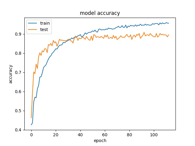
The overall validation accuracy is reaching 89%, which is still pretty impressive without playing with any VGG16 model’s hyper-parameters. With further insight and effort, reaching >95% should not be too difficult.
Now, we can do prediction on the test data.
$ python predict.py --data_dir=flower/sorted --path=flower/sorted/test/*/*.jpg --accuracy
...
[1018]flower/sorted/test/99/image_07934.jpg : 101 (99) ---> 101 (99)
top-5 [101  37  10   5  46] hit True
[1019]flower/sorted/test/99/image_07941.jpg : 101 (99) ---> 101 (99)
top-5 [101  70  10  37   5] hit True
accuracy 0.85
top-5 0.967647058824
The overall test accuracies are,
| metrics | accuracy |
|---|---|
| top-1 accuracy | 85% |
| top-5 accuracy | 96.8% |
If we considered the top-5 accuracy, where the predicted class is in the top 5 prediction, we have achieved 96.8% on the flower classification!
Experiment 3: UEC Food 100 Dataset
At Jonah Group, we used snack watching as a PoC, see the previous post on Snack Watcher using Raspberry Pi 3. The snack classifier is using the classical machine learning techniques on the extracted image features; the accuracy is far from impressive. With the advent of ConvNet, we are hoping to upgrade Snack Watcher+ with a new A.I. brain.
To confirm the potential upgrade, we have located the dataset UEC FOOD 100 (from Food Recognition Research Group at The University of Electro-Communications, Japan) contains 100-kind food photos. Each food photo has a bounding box indicating the location of the food item in the photo but we did not utilize the bounding box for our experiment ConvNet training (see the confusion later in the experiment).
Most of the food categories in this dataset are popular foods in Japan. Therefore, some categories might not be familiar with other people than Japanese. With Toronto’s international food culture, we don’t have a hard time to recognize most of the categories.
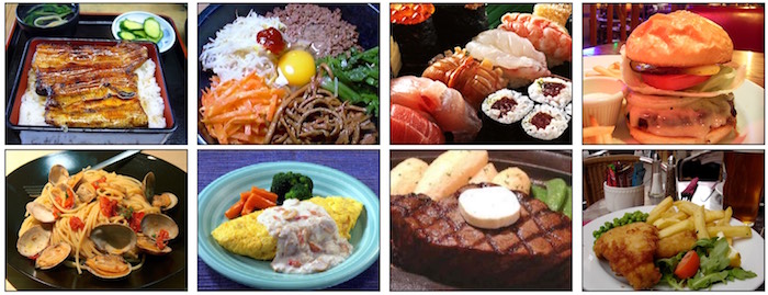
Figure. UEC Food 100 dataset image samples
The sample of the categories,
| id | name |
|---|---|
| 1 | rice |
| 2 | eels on rice |
| 3 | pilaf |
| 4 | chicken-‘n’-egg on rice |
| 5 | pork cutlet on rice |
| 6 | beef curry |
| 7 | sushi |
| … | up to 100 categories |
The food recognition research group latest updates, they achieved 72.26% in the top-1 accuracy and 92.00% in the top-5 accuracy by using DCNN (Deep Convolutional Neural Network) features trained by the ILSVRC2010 dataset.
Each epoch takes 180-200s on NVidia GTX 1070 GPU.
$ python train.py --model=vgg16 --data_dir=food/sorted

...
Weights for "fc1" are loaded
Weights for "fc2" are loaded
Weights for "predictions" are loaded
Found 10006 images belonging to 100 classes.
Found 4355 images belonging to 100 classes.
Epoch 1/100
10006/10006 [==============================] - 200s - loss: 14.9965 - acc: 0.2187 - val_loss: 3.1983 - val_acc: 0.2774
Epoch 2/100
10006/10006 [==============================] - 192s - loss: 5.6558 - acc: 0.2231 - val_loss: 2.6880 - val_acc: 0.3637
...
Epoch 52/100
10006/10006 [==============================] - 189s - loss: 1.2442 - acc: 0.7556 - val_loss: 2.0172 - val_acc: 0.5449
Epoch 53/100
10006/10006 [==============================] - 189s - loss: 1.1892 - acc: 0.7574 - val_loss: 1.9635 - val_acc: 0.5483
The fine-tuning process shows the accuracy is improving over the number of training epoch,
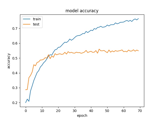
The overall validation accuracy is only 55%. The result is not as impressive comparing with the other experiments. After careful inspection of the prediction failures, we realized that the food picture contains multiple food categories but classified as one specific categories. To add to the challenge, some pictures are hard to say what is the content inside the soup, e.g. the udon noodles. In addition, some food category is bounded to be ambigious, e.g. chinese soup.

Figure. Illustration of food category confusion and challenge
| Id | Category | Source of Confusion |
|---|---|---|
| 1 | rice | has a mixes of side diskes |
| 14 | roll bread | has accompanied with other foods |
| 20 | udon noodles | are completely invisible |
| 91 | chinese soup | is ill defined |
If we considered the top-5 accuracy, where the predicted class is in the top 5 prediction, we can claim 81% accuracy. Of course, we did not beat the UEC research group reported top-5 accuracy of 92%. But they used a more sophisticated combined techniques. In contrast, we are simply using the basic ConvNet transfer learning technique, without much hyper-parameters tuning.
| metrics | accuracy |
|---|---|
| top-1 accuracy | 54.8% |
| top-5 accuracy | 80.8% |
With this food classification result, we are confident to proceed upgrading the Snack Watcher’s recognition ability.
