Preparing Geospatial Data in PostGIS

The Spatial is a popular extension to the traditional database systems. When the data has some spatial attributes, for example a street address or a phone number, we can use the spatial proximity to analyze and calculate their relationships in space. We are usually designating a finite geometric representation and operation on these spatial entities. If you are interested to use the public domain spatial data to solve your analysis problem, read on for a gentle introduction to geospatial data and how to load and use them in PostGIS.

The World as Unified One?

Let’s begin with a curious map projection, Dymaxion Map is a projection of a world map onto the surface of an icosahedron, which can be unfolded and flattened to two dimensions. The flat map is heavily interrupted in order to preserve shapes and sizes.

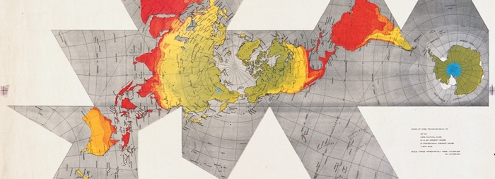
Figure. The Dymaxion map projection can be folded into a Platonic solid of Icosahedron (image credit: Buckminster Fuller Institute )

With this projection, it shows an almost contiguous land mass comprising all of earth’s continents – not groups of continents divided by oceans. This version depicts the earth as “one island” is claiming to help unifying humanity better than other methods of how the map is projected. Another interesting result of using this projection to support analysis, the Early Human Migrations according to mitochondrial population genetics can be explained (see the picture). From this projected perspective, the migration pattern is almost a natural deduction from the spatial arrangement. We may not be able to immediately solve many humanity issues with Dymaxion map. But positively, the spatial perspective does help us to see.

Outlines

In this article, you can expect to begin with the concepts of geospatial data. As always the concepts are supplimented by practical experimentations. Using Docker to quickly spin up a PostGIS instance, you can load the OpenStreetMap (OSM) data into the database. Subsequently, using QGIS to connect with this PostGIS instance, the spatial data can be analyzed and visualized interactively. By the end, you are equipped with a firm perspective of how to prepare geospatial data for the future geospatial analysis.

• The World as Unified One?
• Outlines
• 1. What is Geospatial?
  • 1.1. Representations
  • 1.2. Coordinate Systems
  • 1.3. Map Projections
• 2. Running Dockerized PostGIS
  • 2.1. Persisting Postgres Data
  • 2.2. Creating the Database Container
  • 2.3. (1) Execute psql from localhost
  • 2.4. (2) Execute psql in the PostGIS Container
• 3. Loading OSM Data into PostGIS
  • 3.1. Install Osm2pgsql
    • 3.1.1. From source
    • 3.1.2. For Debian or Ubuntu
    • 3.1.3. For Mac OS X
  • 3.2. Loading Toronto OSM Data
• 4. Displaying PostGIS Data with QGIS

1. What is Geospatial?

The definition of Geospatial consisted of 2 closely related concepts, Geo as in geographic information and Spatial as in representation of objects arranged in space. The relation of a set of spatial coordinates that is reference to a concrete place on earth, we shall say these spatial data are georeferenced; hence, the term geospatial is combined. The best known geospatial application, GIS (Geographic Information System) is recognized as a system of hardware and software used for the input, storage, retrieval, mapping, display and analysis of geospatial data.

Geospatial data come in layers, and each layer has two types of information: graphic and attributes. The former is also called geometric data, and the latter thematic data. Information in the layers can be represented in two forms: raster and vector.

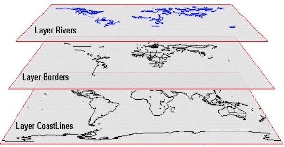
Figure. A typical example of map layers - composition of coastlines, borders and rivers

1.1. Representations

The raster and vector representations are two different geospatial conceptions, used to model the real world. Vector data are graphics, commonly represented by three geometric types: points, lines and polygons. As conformed to geospatial, these graphic objects are situated in georeferenced space according to their coordinates. In the case of raster data, the layer (or space) is considered a grid where each cell (also called a pixel) represents a basic element of information. The raster representation assumed the space exists beforehand, and the object is placed in it. This dichotomy between vector and raster representation left us with two different schools of thought concerning space: in the vector representation, space exists because of the objects, and without the object there is no space; in the raster representation, space is an intuitive idea where objects are placed.

Vector data is composed of points, lines, and polygons. In a vector dataset, each point represents a value at a specific (X,Y) and (optionally) Z point in space. Vector data is best suited for representing discrete features: e.g., the point-of-interests represented by points, the roads represented by lines, and the city boundaries by polygons.

In contrast, raster data is composed of pixels: small, uniformly-sized, grid cells.

Figure. The raster representation of an area showing the color (red, green, blue) values of each cell (pixel). What does the color values mean requires intepretation.

In a raster dataset, each pixel has a value. Pixels representing equivalent data have the same value: Rasters are well-suited for representing continuous data across a broad area: for example, elevation data or temperature measurements. Raster pixels may also be used to represent color values: satellite imagery is an example of this kind of data. Imagine zooming in on an area, allows you to see how each tiny square has a unique value; when put together these pixels make up an image.

1.2. Coordinate Systems

The geometric concept above also applies to geographic space: any point on earth can be described by its latitude, longitude, and (optionally) its elevation. The systems that are used to describe points on the earth’s surface are called Geographic Coordinate Systems (GCS).

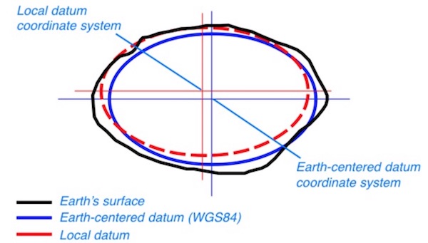
Figure. Illustration of earth is not a perfect ellipsoid. Using WGS 84, the world comes to an agreement of how to address the geographic coordinate on the earth surface.

A GCS uses a mathematically-defined surface called an ellipsoid to represent the earth’s shape. Complex computations based on that ellipsoid define the coordinates that can be used to reference a unique point. There are many coordinate systems, some more common than others: WGS 84 is the one you will see used most often.

1.3. Map Projections

Map Projections allow us to translate locations from a 3D surface (like a globe) onto a flat surface (like a map). The popular imagination to understand a globe projection is like peeling an orange, and then attempting to flatten the peel on a table: it will never perfectly lie flat, and operations such as stretching, cutting, or squashing the peel must be perfored. Map projections must always distort the features they map in some way due to these flattening operations. Different projections might be chosen depending on the way they distort the earth surface.

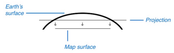
Figure. The concept of map projection - trying to flatten the elliptical earth surface onto a paper. It is necessary to distort in at least one of these metrics (1) Area (2) Direction and/or (3) Distance to the flattening operation.

Geospatial data that has been transformed in order to fit a flat surface is called projected data. The projection used for this transformation is part of the geospatial information (metadata) unique to your data file. Typically for the web mapping, the EPSG 3857 projection, also known as Spherical Mercator or Web Mercator is used for the projection. EPSG 3857 is a projected coordinate system used for rendering maps in OpenStreetMap, Google Maps, etc.

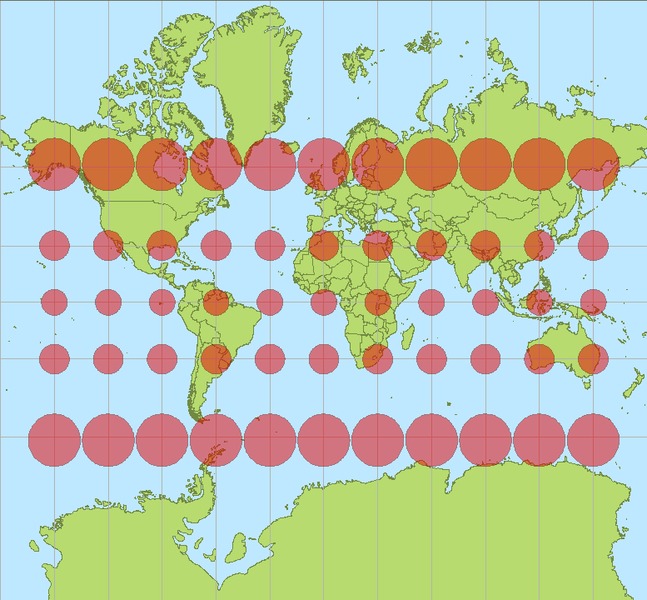
Figure. Web Mercator (EPSG 3857) projection with Tissot‘s indicatrices showing the areal distortion: all disks are of equal area on the globe. (image credit: Wikimedia Commons. Author Stefan Kühn)

2. Running Dockerized PostGIS

PostGIS is the spatial extension to PostgreSQL. Both free open source projects combined conforms to many industry standard (Thanks a millions!). PostgreSQL supports many of the newer ANSI SQL features. PostGIS supports Open Geospatial Consortium (OGC) standards and the new SQL Multimedia Spec (SQL/MM) spatial standard. Learning PostGIS means your knowledge will be useful to other commercial and open source geospatial databases and mapping tools.

One of the big advantage of using Docker is the ability to rapidly build software environment for software system. To help quickly spin up a PostGIS database, we shall use by pre-built PostGIS Docker Image by kartoza/postgis.

• PostgreSQL 10.3
• PostGIS 2.4

The following sections summarized the essential steps of what we needs to run in this article. For further information, you can refer to the excellent tutorial by Alex Urquhart, Setup PostGIS with Docker.

2.1. Persisting Postgres Data

Before we create the database we need to think about how our database info will be stored within Docker. Normally, we specify what’s called a volume in Docker so that database data will be saved outside of the container. With external persistent volume, we can perform backups or upgrades to the database software without losing all your data.

We create a volume container that will be used to persist PostgreSQL database files outside of the the container that runs the database process:

docker volume create pg_data

2.2. Creating the Database Container

Next we’ll use docker run to create the PostGIS container:

docker run --name=postgis -d \
    -e POSTGRES_USER=admin \
    -e POSTGRES_PASS=admin \
    -e POSTGRES_DBNAME=gis \
    -e ALLOW_IP_RANGE=0.0.0.0/0 \
    -p 5432:5432 \
    -v pg_data:/var/lib/postgresql \
    --restart=always \
    kartoza/postgis:10.0-2.4

Lets break down this command part-by-part. More examples of how you can run this container can be found on Docker Hub

• docker run --name=postgis tells Docker our new container will be named postgis
• -d run the container in the background (detached mode)
• -e POSTGRES_USER=admin the -e flag sets an environment variable inside the container. This one is used to configure name of a login role in PostgreSQL that will have superuser (admin) priviliges in the database. You can rename this to whatever you want.
• -e POSTGRES_PASS=admin sets an environment variable that will set the password of the login role to admin. You can set this to whatever you want.
• -e POSTGRES_DBNAME=gis much like you can guess, the environment variable tells the container to create a new database on the server with the name gis. After the database is created then the PostGIS extension will be enabled on it.
• -e ALLOW_IP_RANGE=0.0.0.0/0 tells the container to configure PostgreSQL to accept connections from anyone. If you did not set this then the database would only accept connections from addresses using the Docker networking subnet.
• -p 5432:5432 maps the port 5432 on the host VM to port 5432 on the container. This is required because the database server listens for connections on port 5432 by default.
• -v pg_data:/var/lib/postgresql tells the container filesystem to mount the pg_data volume we just created to the path /var/lib/postgresql. This means that any data that the container saves or creates in that directory will instead be saved in the pg_data volume.
• --restart=always creates a restart policy for your container. Now your container will start every time the Docker virtual machine starts. If this was not set, you would have to manually start the container every time the VM booted up with docker start postgis
• kartoza/postgis:10.0-2.4 tells Docker to pull the kartoza/postgis repository from Docker Hub, using PostgreSQL version 10.0 and PostGIS version 2.4. You can see other versions that are available on Docker Hub

Once the images have downloaded you should then see that the container has started by using docker ps:

CONTAINER ID        IMAGE                      COMMAND                  CREATED             STATUS              PORTS                    NAMES
50ab14716a91        kartoza/postgis:10.0-2.4   "/bin/sh -c /docker-…"   4 seconds ago       Up 3 seconds        0.0.0.0:5432->5432/tcp   postgis

If you want to see log output from postgis container, you can do so by using docker logs.

docker logs postgis

Just for reference, please noted that PostGIS extensions are installed inside the container located at,

/usr/share/postgresql/10/contrib/postgis-2.4

In case we need to execute PostGIS commands to spatially enable the new database (you need to be super user to do this)

createlang plpgsql <dbname>

psql -d <dbname> -f postgis.sql
psql -d <dbname> -f spatial_ref_sys.sql

In order to use psql, you have 2 options (1) use psql from localhost (2) use psql in the PostGIS container.

2.3. (1) Execute psql from localhost

Once you spin up the postgis container, if you have psql client on your host, you can connect to postgis directly because we have exposed the default database port 5432 to the host’s port 5432.

psql -h localhost -U admin gis
Password for user admin:

psql (10.2, server 10.3 (Debian 10.3-1.pgdg90+1))
SSL connection (protocol: TLSv1.2, cipher: ECDHE-RSA-AES256-GCM-SHA384, bits: 256, compression: off)
Type "help" for help.

gis=#

2.4. (2) Execute psql in the PostGIS Container

To enter into the PostGIS container database, run the following command in the terminal. Make sure to replace the PASSWORD, DBNAME and USERNAME parameters with the ones you used when you created the container.

docker exec -it postgis /bin/bash \
    -c "PGPASSWORD=admin psql -d gis -U admin -h localhost"

What this command does is create an instance of the postgis container. Then, it is executing the psql in the container.

Upon successful connection, the psql prompt will be shown.

psql (10.3 (Debian 10.3-1.pgdg90+1))
SSL connection (protocol: TLSv1.2, cipher: ECDHE-RSA-AES256-GCM-SHA384, bits: 256, compression: off)
Type "help" for help.

gis=#

3. Loading OSM Data into PostGIS

OpenStreetMap (OSM) is a collaborative project to create a free editable geospatial data of the world. The OSM crowdsourced data is made available under the Open Database License, such that the data can be freely share, modify and use in a database. Thanks to this free data source, many social and humanitarian mapping projects are made possible. We shall use the OSM data in the following sections.

3.1. Install Osm2pgsql

We need the osm2pgsql program installed to load OSM data into PostGIS.

3.1.1. From source

Prerequisite lists are listed in the osm2pgsql README The main dependencies to be aware of for old distributions are a C++11 compiler and Boost 1.50 or later.

3.1.2. For Debian or Ubuntu

apt-get install osm2pgsql

3.1.3. For Mac OS X

With Homebrew

brew install osm2pgsql

3.2. Loading Toronto OSM Data

OSM data can be downloaded freely from Geofabrik Download Server. However, for our experiementation only to cover Toronto area, we take an easier (much smaller in size) route to only download the Toronto.osm.pbf file from OSM extracts for Toronto.

Then using osm2pgsql, we can load the Toronto OSM data into PostGIS (Note: the password is specified from the PGPASSWORD).

There is an interesting post: http://weait.com/content/build-your-own-openstreetmap-server It says, ‘you must use slim mode’.

PGPASSWORD=admin osm2pgsql --slim -c -d gis --host localhost -U admin Toronto.osm.pbf

It proceeds to convert OSM data to PostgreSQL statements for loading. As a note, we observed the OSM data is in 3857 (Spherical Mercator) projection, as shown in the logs.

osm2pgsql version 0.96.0 (64 bit id space)

Using built-in tag processing pipeline
Using projection SRS 3857 (Spherical Mercator)
Setting up table: planet_osm_point
Setting up table: planet_osm_line
Setting up table: planet_osm_polygon
Setting up table: planet_osm_roads

... skipped

Osm2pgsql took 67s overall

After the OSM data loaded, we can use pgAdmin, which is the most popular administrative tool for PostreSQL or PostGIS. For example, we are using pgAdmin4 to look into the gis database public schema planet_osm_polygon table here.

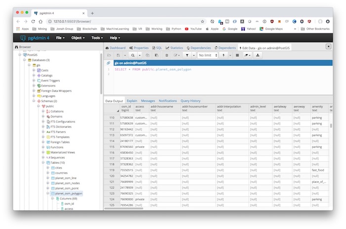
Figure. Using pgAdmin4 to select from planet_osm_polygon table. We can see the planet_osm_polygon is a big collection of many types of polygons. We have noticed the amenity column can be used to select specific type of polygons, such as “parking”.

4. Displaying PostGIS Data with QGIS

QGIS is a free and open-source cross-platform desktop geographic information system (GIS) application that supports viewing, editing, and analysis of geospatial data. We shall use QGIS to display the Toronto OSM data loaded in PostGIS.

We should be able to add the connection to PostGIS in the browser panel in QGIS. Right click the PostGIS icon and click “Create New Connection”, and enter the database connection parameters we used in the section 2 docker run command. If using Docker VM, the “Host” parameter will the the IP of the Docker VM (running docker-machine ip in the terminal window)

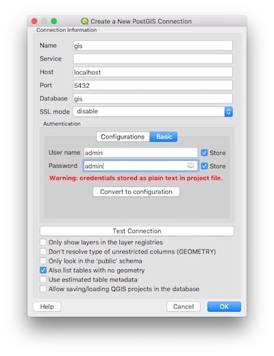
Figure. Using QGIS to create a new PostGIS connection. We are using the database creation settings when we do docker run on the PostGIS container instance. The admin password is intentionally shown here for illustrative purpose.

In the screenshot below, it shows the loaded OSM data of Toronto area with planet_osm_polygon and planet_osm_road layers added.

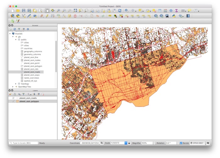
Figure. Simply right-click on a PostGIS table to be added as layer to display. After adding the layer, you can tune the layer by enhancing the various graphics display properties, such as colors, line wide, fill patterns etc.

After some inspection on the planet_osm_polygon table, we would like to reduce the clutters of displaying too many polygon types, we can filter to select a subset of polygon types from the DB Manager query.

First, we select all the non empty boundary polygon by

SELECT osm_id, boundary, name, way_area, way
    FROM planet_osm_polygon
    WHERE boundary is not NULL;

Open the DB Manager -> Query Layer icon, and execute the selection to load the results into the neighborhoods layer.

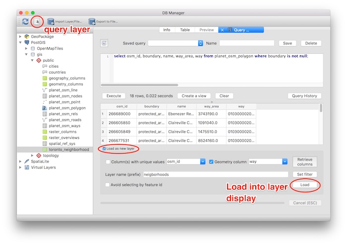
Figure. Using the DB Manager->Query Layer dialog to use SQL statement to select a subset of polygons from planet_osm_polygon table. After the query, you can load the results as a display layer. In this illustration, we have selected the non-empty boundary polygons.

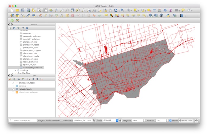
We can see the neighborhoods layer display.

Continue with more selections, we select all amenity='parking' polygons by

SELECT osm_id, amenity, way_area, way
    FROM planet_osm_polygon
    WHERE amenity='parking';

Once again, open the DB Manager -> Query Layer icon, and execute the selection to load the results into the parking layer.

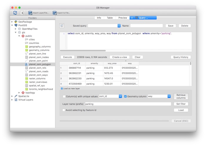
Figure. Using the DB Manager->Query Layer dialog to use SQL statement to select a subset of polygons from planet_osm_polygon table. After the query, you can load the results as a display layer. In this illustration, we have selected the parking polygons.

Then, we can see the parking layer display on top of the neighborhoods layer.

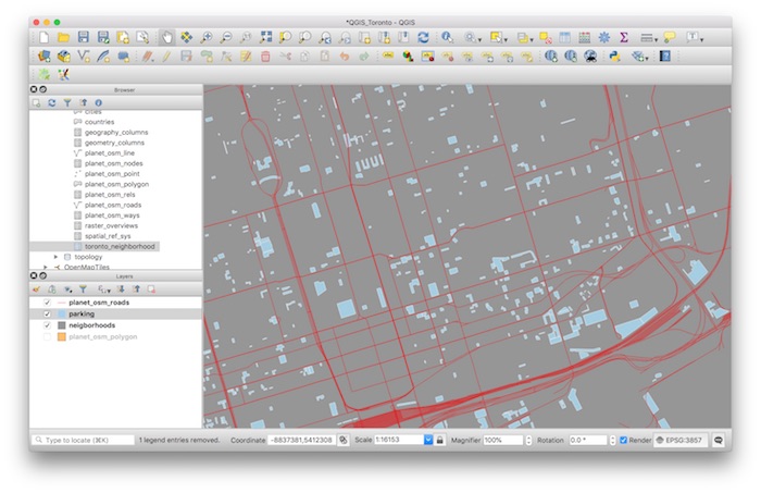
Figure. After fine tuning the planet_osm_polygon selections to only display neighborhoods and parking, we get the clear visualization of the Toronto download parking areas.

With the addition of geospatial data, we can ask deeper spatial analysis questions, for example, finding all the parking within 100 meters from planet_osm_road named “King Street” within the neighborhoods of “Toronto”. But we shall expand the analysis topics until the next article.

Enjoy your totally open and free geospatial technology stack!