artwork by Style of Byzantine mosaics transfer to a global projected map
Geospatial Granular Computing
Granular Computing can be conceived as a framework of theories, methodologies, techniques, and tools that make use of information granules in the process of problem solving. In particular, the granular computing has been implicitly used in geospatial representation and processing in order to conquer the complexity and diversity of a large geographic data set.
[2024/10/05] We can listen to this article as a Podcast Discussion, which is generated by Google’s Experimental NotebookLM. The AI hosts are both funny and insightful.
images/geospatial-granular-computing/Podcast_Geospatial_Granular_Computing.mp3
Starting with the questions on “what is granular computing?” and “why is that important for geospatial problem solving?”, we shall step back from the long history of specific problem solving, to re-imagine a theory and to re-structure the spatial constructs. Using the ideas from granular computing, we shall re-discover a solution to geospatial problem. For concrete illustration of the theory, an important geospatial problem - Geocoding is chosen.
Geocoding is the process of taking an address or named location and returning a longitude and latitude. With a georeferenced longitude and latitude, many geospatial analysis and processing are made possible, such as mapping, routing, proximity searches, etc. Since our focus is on “georeferenced” spatial parts, we shall assume spatial is meant geospatial from this point. Additionally, the theory formulated in this article, can be extended to other geospatial analytic problems.

Figure. Geocoding is the process of converting addresses (like a street address) into geographic coordinates (like latitude and longitude), as if the dropped red-pin is the result of the geocoded address.
Explaining the theory of geospatial granular computing, we shall explore the following topics.
As a side note, another unification effort is the theory based on Geospatial Semantic Web [ZhZhLi15]. Geospatial semantic web is using RDF representation of spatial data and GeoSPARQL as query language. The semantic representation can provide infrastructure to a knowledge engine to support powerful reasoning and information retrieving from heterogenous data sources. However, the downside of representing structured geospatial data in these languages can result in inefficient data access, which is the main reason that we stay away from this approach.
Thinking in Granular Computing?
In a philosophical sense, granular computing has been foundational to human ability to analyze the complex world, by abstracting into a connected and hierarchical levels of granularity. To help reasoning with a specific interest, we come to switch among different granularities. For instance, if we are planning for a long distance trip, we would first plan in the macro country-level travel. Then we assume in the context of destination country, we come to switch to micro city-level, and then street-level granularity to reach a point of interest. By focusing on different levels of granularity, the relevant levels of knowledge can enhance understanding of the inherent knowledge structures. The structural system thinking is thus essential skill in human problem solving and hence has a very significant aspect of intelligence, in this case spatial reasoning.
From the book, A Unified Framework of Granular Computing (chapter 17 of [PeSk08]), Yiyu Yao presented the granular computing offers these three unified perspectives across problem domains.
- Philosophical perspective, offers a new world view that leads to structured thinking.
- Methodological perspective, deals with structured problem solving.
- Computational perspective, concerns structured information processing.
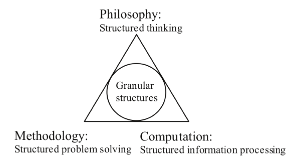
Figure. The three perspectives of Granular Computing forming a conceptual framework to unify cross problem domain principles. (image credit: Yiyu Yao)
Most importantly, Yao argued the important advantage of converging different domains into a share conceptual framework using granular computing, can extract high-level commonalities of different domains and synthesize their results into an integrated whole by ignoring the particular low-level details. Subsequently, the shared concepts make explicit where the ideas hidden in domain-specific discussions in order to arrive at a set of domain-independent principles.
By overlaying the granular computing concepts onto the geospatial domain, the former integration of the three perspectives on system thinking, results in a holistic understanding of geospatial processing that emphasizes structures embedded in a web of granules.
Spatial Granule
A complex spatial problem consists of interconnected and interacting spatial parts. Each spatial part can consist of other parts. For each spatial part or a group of parts may be considered as a spatial granule. These spatial granules will become a primitive notion of geospatial granular computing. The physical meaning of spatial granules may be made clear when a particular spatial processing is considered. In modelling complex geospatial systems, granules may be structured into the spatial layers at different levels.
In geocoding system, granules may be varying with layers at different levels, for example, a country as a granule in the country layer or a province as a granule in the province layer. In any layer, granules can be abstractly represented various divisions of spatial entities. Consider the application of the geocoding system, a spatial granule can be considered as a focal point of interest at a certain stage of locating a requested address.
For the spatial granule’s form, we shall use vector representation to describe their geometry. The geocoding system is not only concern about polygons, such as countries and regions. It also includes points and polylines, when the geocoding calculation is down to the street level address.
Geospatial Granular Structure
In a map, geographic data is usually organized into layers. Each layer represents some consistent concept about geographic features. Geographic features can be classified into three key geometric data types, namely point, polyline and polygon. Correspondingly, these geometries can represent location feature, linear feature or areal feature. Many data types such as label, measurement and quality can be attributed to each feature. Without losing generality, the map model adopts one hierarchy of combinations.
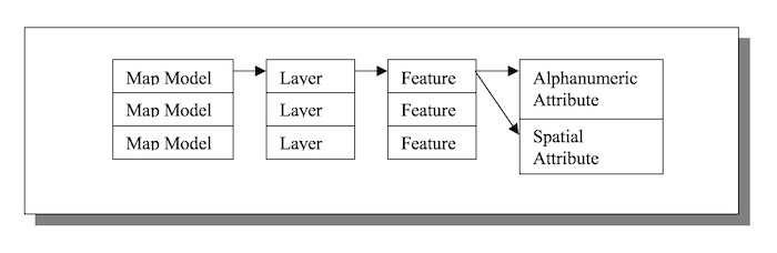
Figure. The geospaital granule structure of a typical map model.
For each map model, it collects many layers. For each layer, it composes many features. For each feature, it defines spatial and alphanumeric attributes. The combined spatial and alphanumeric attributes select graphics representation and meanings. This conceptual view is the basis of the geospatial granular structure.
This is one of many possible methods to describe a concrete map model. But the world view in terms of granules and multiple levels of granularity represented by layers, forming a connected and hierarhical structure are the principles of granular computing.
Geospatial Granule
To qualify as a geospatial granule, the granule must be a georeferenced spatial entity. For the spatial entity to be computable, we need to represent the spatial property as geometric structure. We choose the vector representation of our spatial entities, a Point is represented by its tuple of coordinates. A Polyline or a Polygon are represented by structures (lists, sets or arrays) on the Point representation. There exists a large number of variants to represent Polyline and Polygon vectors. For a comprehensive overview of all popular vector representations, see Chapter 2 in [Westra15].
Note: We intentionally avoid using Open Geospatial Consortium (OGC) WKT (well-known text) format for simple feature representation; even though OGC is extremely important in the industry. The precise geometry representations are little value in our discussion here.
For simplicity, the following vector representation is used:
- A Point is represent by \((x,y)\) coordinate.
- A Polyline is represented by a list of points \([p_1, …, p_n]\), each pi begin a vertex. Each pair \((p_i, p_{i+1})\), with \(i < n\), represents one of the polyline’s edges.
- A Polygon is also represented by a list of points. The notable difference is that the list represents a closed polyline, and therefore the pair \((p_n, p_1)\) is also an edge of the polygon.
In a textual context, we use the following notation to specify a spatial value:
| Spatial Type | Textual Notation | Textual Examples |
|---|---|---|
| Point | (x,y) | (4,7) |
| Polyline | [{point}] | [(4,4),(6,1),(3,0),(0,2)] |
| Polygon | [{point}] | [(4,4),(6,1),(3,0),(0,2),(4,4)] |
.
Granular Relation
The important step to formulate the theory, we need to model the atomic granule where the information processing originated. A Granular Relation is the atomic represention of the spatial granule. Since this relational representation is the theoretical foundation to derive the theory, we shall describe the granular relation with a better mathematical precision and generality.
The relation is modeled as a tuple which composed of both alphanumeric and spatial attributes. We adopt the following conventions: we use \(ST\) for a spatial attribute type, and \(AT\), \(AT_1, AT_2, …\) for a alphanumeric attribute type. Capital letters such \(A\), \(A_1, A_2, …\) are used for alphanumeric attribute names, and \(S\), \(S_1, S_2, …\) for spatial attribute names. Values are denoted by lower case letters.
A Layer can formally define as a granular relation and it collects a set of granular tuples (aka. atomic granule). As an example of granular tuple, \((A_1:a, A_2:b, S:r)\) will designate a feature with spatial attribute \(S\) with value \(r\) and with two alphanumeric attributes \(A_1\) and \(A_2\) with respective values \(a\) and \(b\).
To qualify as as spatial granule, we do not require the existence of alphanumeric attributes (e.g. \(\{(S:r)\}\) represents a layer including a single feature). However, a layer must have at least one spatial attribute. To define more formally a layer, we follow the complex objects approach in [AbBe95] and map modeling in [ScVo89]. Layers are typed granules defined as follows.
We assume a finite set of attribute names (spatial or not), a given set of non-spatial domains \(\{D_1, …, D_n\}\) and a given set of spatial domains \(\{\triangle_1, …, \triangle_m\}\), where \(\triangle_i \in \mathbb{R}^2\).
Types are constructed from domains, attribute names, and the set {} and tuple () constructors. Each layer is an instance of a type which is defined as follows:
- if spatial \(\triangle\) is a domain, then \(S:\triangle\) is a spatial type.
- if \(AT_1, …, AT_n\) are types and \(A_1, …, A_n\) are attribute names not used in any of them, then \((A_1:AT_1, …, A_n:AT_n)\) is an alphanumeric tuple type.
- if \(AT\) is a type and \(A\) an attribute name not used in it, then \(\{A:AT\}\) is a set type.
- if \(AT\) is a type and \(A\) a name not used in it, then \(A:AT\) is a named type.
We illustrate this definition by examples of layers and associated types:
- \(\{S:r, S:s\}\) of type \(\{S:ST\}\)
- \(\{(A_1:a, A_2:b, S_1:r_1, S_2:r_2)\}\) of type \(\{(A_1:string, A_2:string, S_1:\triangle, S_2:\triangle)\}\)
- \(\{(A_1:a, A_2:b, S:\{r_1,r_2,r_3\})\}\) of type \(\{(A_1:string, A_2:string, S:{\triangle})\}\)
By combining the previously described geospatial granules and their relations,
we can generate our geospatial granular structure.
We define a layer name Map as a collection of geographic Layer.
A Layer is a collection of geographic Feature. At the atomic level, we shall have the Feature relation defined.
Below is a generic definition of a map model:
- Map = {Layer}
- Layer = {Feature}
- Feature = \((\{A_i:AT_i\}, S:\triangle)\)
where \(\{A_i:AT_i\}\) denotes an enumeration of named types (the alphanumeric attributes). \(AT_i\) translates to a basic alphanumeric type that is supported by geospatial system. \(S\) denotes the name of a spatial attribute whose type is \(\triangle\). \(\triangle\) can be one of the geometric type of Point, Polyline or Polygon that are supported by the geospatial system.
As an illustration, the following geospatial granular structure can be defined:
- The set of alphanumeric domains is {NUMBER,STRING,BOOL}
- The set of spatial domains is {\(\triangle\)}
- The attribute name set is {Name,Population,Area,Streetid,Class,Region,Shape}
The granular relations are,
- City = \((Name:STR, Population:NUM, Area:NUM, Region:\triangle)\)
- Street = \((Streetid:NUM, Name:STR, Class:NUM, Shape:\triangle)\)
The granular layers are,
- City Layer = {City}
- Street Layer = {Street}
The map model is formed by,
- Map = {City Layer, Street Layer}
Granular Algebra
To continue with the computational perspective, a granular algebra is formally defined to enable granular processing via a set of well-defined operators. The definition of granular algebra is used to specify the operational semantics between the domains. We are referring to many results from the literature for guiding the development of such algebra. The geospatial query language must follow the semantics defined by the granular algebra in order to retain applicability and closure of the operations.
Note: Geocoding process does not require the full set of granular algebra defined here. These definitions can be extended to perform additional geospatial analytics.
The granular algebra starts from a view of relational algebra as a many-sorted algebra. This type of algebra is well developed in many systems [AbBe95] [GuSc93a] [GuSc93b] [ScVo89], including some popular commercial spatial database systems [RiMiVo02] [ScVo92]. The objects of the algebra are atomic values such as string, number or boolean values as well as relations. The operators of the algebra include arithmetic operators (e.g. addition, subtraction) on numbers as well as the relational operators (e.g. selection, join).
Following the geospatial granular relation, the spatial attribute is part of the relation. Spatial types and operators are embedded in the algebra as part of the sorted object. The spatial types encapsulate geometric representation such as point, polyline and polygon, that we have defined in geospatial granule section. Furthermore, the specific spatial operators are introduced for accessing and operating on these spatial attributes. We shall only have a glimpse at the spatial operations here, another article should be devoted for the full treatment of this topic.
Our granular algebra begins with the following set of sorts:
| Domain Type | Description |
|---|---|
| NUM | numbers, including integer or real numbers |
| STR | alphanumeric string values |
| BOOL | boolean values |
| REL | relations |
| ST | spatial values |
.
A sample list of operators in the granular algebra is given. The list is grouped into 3 classes of operators. The first class comprises all the usual operations of a relational database system plus some additional operators. The second class contain spatial operators. The remaining class contain composite operators.
Table of relational operator class:
| Operator Signature | Operator Symbol | Description |
|---|---|---|
| \(NUM \times NUM \to NUM\) | \(+, -, *, /\) | standard arithmetic operators |
| \(BOOL \times BOOL \to BOOL\) | and, or | standard boolean operators |
| \(BOOL \to BOOL\) | not | standard boolean operators |
| \(REL \times REL \to REL\) | union, intersect, difference, cross, extend, join | binary relational operators |
| \(REL \times AT_i \to REL\) | select, project | unary relational operators |
| \(NUM \times NUM \to BOOL\) \(STR \times STR \to BOOL\) \(BOOL \times BOOL \to BOOL\) |
\(=, \lt, \gt, \le, \ge, \neq\) | comparison operators |
| \(STR \times STR \to BOOL\) | like, match | string matching operators |
| \(REL \to NUM\) | count | statistical operators |
| \(NUM*\) | sum, avg, min, max | statistical operators |
.
Table of spatial operator class:
| Operator Signature | Operator Symbol | Description |
|---|---|---|
| \(ST \to NUM\) | diameter, length, area | spatial metric computation operators |
| \(ST \to ST\) | bound, center, buffer | spatial representation operators |
| \(ST \times ST \to BOOL\) | \(=, \neq\), inside, outside, intersect, near | spatial predicate operators |
| \(ST \times AT_i \to ST\) | select, project | spatial object selection operators |
| \(ST \times ST \to ST\) | union, window, clip, overlay | binary spatial operators |
| \(ST \times ST \to NUM\) | dist | binary metric operator |
.
Table of composite operator class:
| Operator Signature | Operator Symbol | Description |
|---|---|---|
| \(REL* \to REL\) | select:into:from, select:into:from:where, select:into:from:where:rankby |
extend operators to support SQL alike operation |
.
Geocoding Query
After equipping with all the formulation with geospatial granular relation and algebra, we are finally ready to breathe live into the geocoding process. The layers are defined as:
Country = (Id:NUM, Name:STR, ShortName:STR, Shape:ST)
Region  = (Id:NUM, Name:STR, ShortName:STR, Shape:ST)
Postal  = (Id:NUM, Code:STR, Shape:ST)
City    = (Id:NUM, Name:STR, Shape:ST)
Street  = (Id:NUM, Name:STR, Shape:ST)
Place   = (Id:NUM, Name:STR, Shape:ST)
Geocoding queries are composed according to the granular algebra. For these example compositions, the expressions are written in a functional programming style; however, the precise language will be not defined in here.
| Query ID | Layer | Granular Algebra |
|---|---|---|
| [Geocode-Country] | Country | (project Country (select (Country.Name match $country) or (Country.ShortName match $country))) |
| [Geocode-Region] | Region | (project Region (select (Region.Name match $region) or (Region.ShortName match $region) and (Region.Shape intersect Country.Shape))) |
| [Geocode-Postal] | Postal | (project Postal (select (Postal.Code match $postal) and (Postal.Shape intersect Country.Shape))) |
| [Geocode-City] | City | (project City (select (City.Name match $city) and (City.Shape intersect Region.Shape))) |
| [Geocode-Street] | Street | (project Street (select (Street.Name match $street) and (Street.Shape intersect City.Shape))) |
| [Geocode-Place] | Place | (project Place (select (Place.Name match $place and (Place.Shape intersect City.Shape)))) |
.
Geocoding process can be easily observed as a process that is refining a sequence of progressively smaller spatial granules to a atomic spatial granule. However, the granular computing allows to define and process layers flexibily by using the set of spatial/relational operators. As a result, the granular computing is shown to be a powerful conceptual framework to express a geospatial problem and formulate a solution.
Preview of Geospatial Analytics
To preview the full utility of the granular algebra, the queries can go beyond the geocoding process. We can perform geospatial analytics with the granular structure and processing.
The following illustrates a few geospatial analytic queries, can be expressed with our geospatial granular computing.
- Find the “X” street in “C” city and fall with the UI’s window.
(project Street
  select    (Street.Name match “X”)
        and (City.Name match “C”)
        and (Street.Shape intersect City.Shape)
        and (Street.Shape inside UIWindow.Shape))
- Find the “X” street that is close to intersection of “Y” and “Z”.
(project Street
 select     (Street.Name match “X”)
        and (InterLayer.Name match “Y" and "Z”))
        and (Street.Shape near InterLayer.Shape))
- Find the “X” street in “US” and it is close to River “R”.
(project Street
 select     (Street.Name match “X”)
        and (Country.Name = “US”)
        and (River.Name match “R”)
        and (Street.Shape inside Country.Shape)
        and (Street.Shape near River.Shape))
- Find all the street that is 1 km away from my home.
(project Street
 select     (Place.Name match “my home”)
        and (Street.Shape intersect
             (bound (center Place.Shape) 1000)))
Final Notes
We have presented the essential concepts of granular computing applied to the geospatial domain. Although we avoided using any existing GIS technologies and standards in here, for those readers, who is well-versed with the state-of-the-art GIS, can easily draw the connections to the actual geospatial implementation. By digesting the abstract discussion, we can concentrate on the high-level commonalities of the structural thinking in granular computing; subsequently, we can synthesize similar structural thinking to other domains to solve interesting spatial problems.
References
- [AbBe95] S. Abiteboul and C. Beeri, “On the power of languages for the manipulation of complex objects”, The VLDB Journal, vol.4, no.4, pp. 727-794, 1995.
- [GuSc93a] R.H. Guting and M. Schneider, “Realms: A Foundation for Spatial Data Types in Database Systems”, in Advance in Spatial Databases (SSD’93). Lecture Notes in Computer Science No. 692, 1993, Springer-Verlag, Berlin.
- [GuSc93b] R.H. Guting and M. Schneider, “Realm-Based Spatial Data Types: The ROSE Algebra”, Tech. Report 141, Fern University, Hagen, Germany, 1993.
- [PeSk08] W. Pedrycz, A. Skowron, V. Kreinovich (Editors), “Handbook of Granular Computing”, 2008, Wiley-Interscience, ISBN:9780470035542.
- [RiScVo02] P. Rigaux, M. Scholl and A. Voisard, “Spatial Databases: with Application to GIS”, Academic Press, Morgan Kaufmann Pub., 2002. ISBN:9781558605886
- [ScVo89] M. Scholl and A. Voisard, “Thematic Map Modeling”, in Design and Implementation of Large Spatial Databases (SSD’89). Lecture Notes in Computer Science No. 409, 1989, pp. 167-192, Springer-Verlag, Berlin.
- [Westra15] E. Westra, “Python Geospatial Analysis Essentials”, 2015, Packt Publishing, UK. ISBN:9781782174516
- [ZhZhLi15] C. Zhang, T. Zhao and W. Li, “Geospatial Semantic Web”, 2015, Springer, Switzerland. ISBN:9783319178011