Model of Spatial Construction

The heart of a spatial reasoning system is utilization of spatial knowledge. With proper represented spatial knowledge, the task of spatial reasoning is made intuitive, flexible and practical. This article introducing the concept of Spatial Construction, which is the theory of deriving the spatial knowledge. The strength of the theory is it’s intuitive foundation that allows flexible and practical algorithmic construction of spatial knowledge. We shall concentrate on setting up the foundation of spatial construction. The other concern for spatial reasoning, which is how to utilize the spatial knowledge effectively and efficiently, we leave that until another article to elaborate.

Towards the end, we shall introduce PyDelaunay (https://github.com/bennycheung/PyDelaunay) as a practical spatial construction. It is an efficient Python implementation of Voronoi/Delaunay Tessellation, which can be served as the Basic Map of the neighbourhood concept.

Model of Spatial Reasoning

Spatial reasoning is described in terms of a generic solution to many spatial problems. Considering that spatial knowledge is represented as a set of entities and a set of relations, spatial reasoning is a knowledge increasing process which is designed to use spatial primitives to deduce more and more specific relations between any two entities. For example, in an environment \(G_s\), the possible solution space may be described by all possible connectivities between \(v_a\) and \(v_b\).

Although it is not a specific relation between \(v_a\) and \(v_b\), the spatial reasoning process tends to produce more specific relations between \(v_a\) and \(v_b\). In this case, “\(v_a\) is related to \(v_b\) via \(v_c\)”, is a new relation and it is more specific than the complete graph connections.

The deduction of this specific relation may be a knowledge intensive process or pure algorithmic process. In each case, however, this newly deduced relation is defined as a spatial reasoning step. After the deduction of this new spatial relation, it may be immediately recorded inside the knowledge base. The new piece of knowledge may enhance other steps of spatial reasoning as long as the relation, “\(v_a\) is related to \(v_b\) via \(v_c\)”, still holds in the knowledge base.

Spatial reasoning can be further divided into two subprocesses: Spatial Construction and Spatial Utilization. Spatial construction is the foundation for all spatial reasoning activities since it provides ways to represent space and spatial semantics. Spatial utilization is the actual process, using spatial constructs and spatial primitives, to construct some very specific relations. Spatial construction can be viewed as a generic representation for any application but the spatial utilization is more application specific. The application may impose its domain knowledge which affects spatial utilization. Although this model separates these two subprocesses, they should be viewed as complementary processes to each other as illustrated.

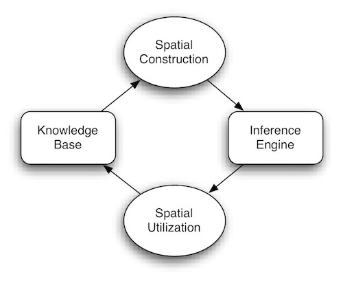
After spatial construction, the base knowledge can be immediately applied in the utilization step. After the utilization step has deduced new traversal information, it may reconstruct some of the base knowledge. To start the construction process, an external procedure is needed. This procedure may be a predefined knowledge base or some knowledge acquisition process.

The traditional framework of reasoning consists of two important parts, which are the knowledge base and the inference engine. The definition of spatial reasoning as a process does not deviate from this fundamental construct but elaborates on the structure by incorporating specific processes. These specific processes are driven by intensive spatial knowledge. Therefore, this model is not a new type of reasoning mechanism but a new process control to serve as a supporting mechanism for the needs of spatial reasoning.

Spatial Construction

The natural grouping of spatial entities is the basis of a spatial construction concept. The original reasoning scheme, which separates knowledge base and inference engine, is still applicable. However, the new proposed scheme suggests that the spatial knowledge base is indexed by its inherent spatial knowledge, as illustrated.

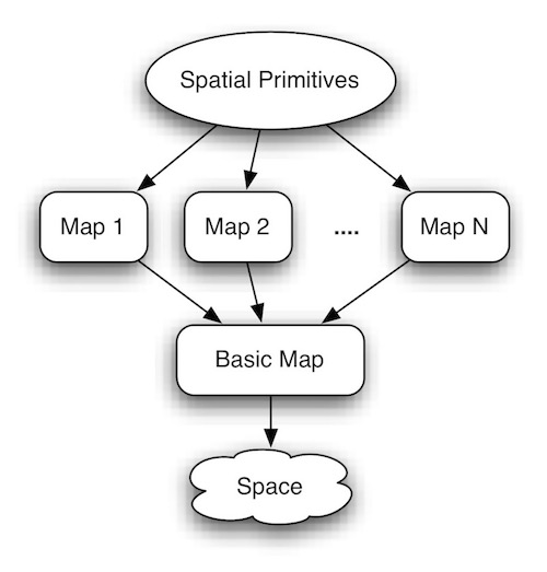
This basic indexed space is called the Basic Map. This basic map not only captures the neighbourhood nature of space but also provides a fast processing structure for geometric information.

After a basic map is constructed, a variety of other maps (including topology, structure, etc.) can also be constructed from the multi-facet and hierarchical nature of space. Moreover, based on the requirements of applications, specialized maps can also be derived. The notion of starting from one basic map, from which all other maps are derived, is supported by recent AI cognitive research. The important point is that every map is derived from the basic map such that maintenance is possible. Also, once the basic map has been changed, through a derivation scheme, other maps can be updated automatically and systematically. This is because all the spatial primitives can be efficiently implemented based on these maps.

This approach does not mean to break down the traditional reasoning scheme but to create an escape mechanism for special needs identified for spatial reasoning. The definition of spatial primitives is exported to the reasoning system. Whenever the system encounters these primitives, it hands the task to the specialized spatial reasoning engine to execute these primitives. This escape mechanism is reasonable since it has been demonstrated by most of the graphical systems, e.g. OpenGL as implemented in hardware, which is closely related to geometrical processing with triangles. The graphical application built on top of OpenGL, can be programmed with high-level graphical primitives. This design not only enhances the performance but also simplifies the modelling of the application domain.

The dynamics of spatial reasoning can be demonstrated by high level application semantics. Intelligence cannot easily be seen in points, lines and polygon processing but through their combined structures and relations. However, the generality is maintained within the basic map.

In order to accommodate higher level spatial reasoning tasks, there may be more layers on top of a set of spatial primitives. These layers, most likely, are application dependent. The basic constructs will not differ between applications since these deal with space directly, with nothing being related to the application’s spatial attributes. Whenever spatial attributes are imposed on top of these constructs, much intelligent reasoning can be realized.

Basic Spatial Constructs

It is clear that there is a need for techniques that exploit sets of all possible spatial properties to solve spatial problems. The associated structure should not be so general that spatial properties are lost. In order to capture both intentional and extensional semantics for spatial reasoning, there are four basic spatial constructs:

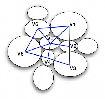
• Spatial Cells : The continuous space has to be represented by a set of discrete units, called spatial cells. A finite amount of area is represented by a spatial cell, usually referenced by an unique identifier. As illustrated, the Spatial Cells are regions that covering some portion of the represented space. If the spatial cells are connected directly, we can put an edge between them to indicate spatial connectedness.

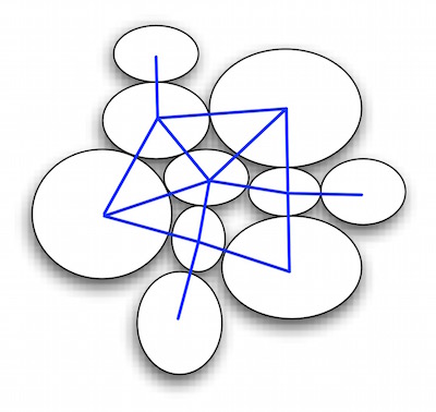
• Neighbourhood : The determination of neighbourhood corresponding to spatial sorting is a prerequisite for making the continuous space into discrete computational units. Usually, the neighbourhood is determined by the relative position of spatial cells. As illustrated, the Neighbourhood of \(V_0\) is composed of the set of \({V_1, V_2, ..., V_6}\).

Sometimes, if two spatial cells share a common boundary then this can also be refered to as a neighbourhood. The intentional semantics is embedded in the use of neighbourhood because an object can uniquely be described by its position relative to its neighbour.

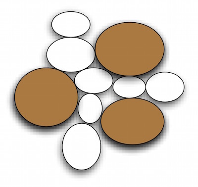
• Categorized Space : A set of spatial cells can be aggregated together and referenced by an unique identifier. These aggregated regions are referred as a categorized space since a group of spatial cells is manipulated as an unit at this level. As illustrated, the Categorized Space classified the spatial cells into the obstacles (coloured brown) and free spaces (coloured white).

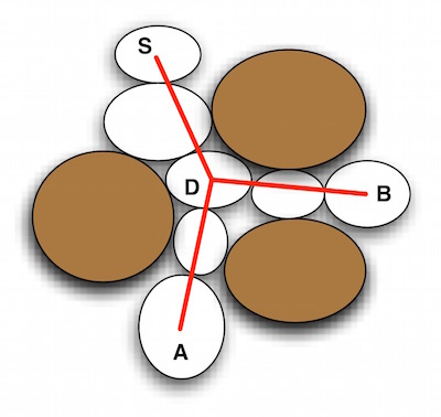
• Maps : Maps can be visualized as the representation of the complete space which can be in either an exact form or in an abstracted form. The maps provide a global view of the whole problem space. As illustrated, the Free Space Map composed of the key decision points. \(S\) is the source and \(D\) is the decision point. We can potentially exit from \(D\) to either \(A\) or \(B\) points.

As a result, the extensional semantics are embedded in the use of maps because use of the maps can prune out many unreasonable spatial selections.

Spatial constructs fit into the former concept of spatial reasoning as a process for deducing more and more specific relations. The neighbourhood information is the most fundamental relation for meaningful knowledge. The construction of neighbourhoods is similar to constructing a possible computational relation of discrete spatial entities. It represents localized decisions that can be considered in spatial reasoning. The categorized space is the traversal information that combines these relations to form a more specific relation. The global knowledge is enhanced in the utilization of the maps. Furthermore, the availability of maps can actually enhance local decisions.

Neighbourhood as a Basic Map

The neighbourhood structure should be the basic map of a spatial reasoning system. A sound notion for neighbourhood of an object is essential for analyzing and determining a local optimal decision. This type of locality is desirable because it can enhance the computational power by limiting the number of choices. Any characterization or comparison of spatial entities must be in terms of the relative spatial arrangement. However, the inherent difficulty of deciding on a set of neighbourhoods appears in either of two ways. Firstly, any inference about relations between spatial entities can be made only if there is a known process with a known typing. However, in general, such prior knowledge or model of typing process is usually unavailable. Secondly, global features of spatial entities are important in the perception of their relations. However, taking global features into account implies a top-down approach, and hence is dependent on the availability of a model. Without a model or any prior knowledge of a set of objects, any inference about the structure and relationship must be data driven. Structural descriptions, such as neighbourhoods, must be built using the relative positions of the spatial entities. Therefore, a sound notion of neighbourhood is necessary.

All of the previous attempts to define neighbourhoods suffer the same problem: the inability of dealing with varying density in the spatial set. The performance of these methods depends upon the values of the parameters. Hence, there may always be a need to tune the parameters for best performance for a given density. However, it should be observed that humans find it easy to identify neighbourhoods and the neighbours of a spatial entity in a wide variety of patterns, including those having varying density. This would suggest the existence of a general parameter free concept of neighbourhood. In the field of Computation Geometry, the Voronoi tessellation is used to construct such a basis neighbourhood structure which shows promise of being able to overcome many of the former problems. Therefore, the basic map of a new spatial reasoning system should have the same capabilities as found in the Voronoi tessellation.

Voronoi/Delaunay Tessellation as Basic Map

The set of all points closest to a given point in a point set than to all other points in the set is an interesting spatial structure called a Voronoi Polygon for the point. The union of all the Voronoi polygons for a point set is called Voronoi Tessellation.

Many applications have been found based on the neighbourhood information provided by this tessellation. The dual of Voronoi tessellation is Delaunay Tessellation, also referred to as Delaunay Triangulation or Triangulated Irregular Network (TIN), which are lines drawn between points where their Voronoi polygons have an edge in common.

Delaunay tessellation is the most fundamental neighbourhood structure because many other important neighbourhood structures, such as, Gabriel Graph, Relative Neighbourhood Graph and Minimal Spanning Tree, can be derived from it.

PyDelaunay is a Python implementation of an incremental algorithm, for the construction of Delaunay Tessellation. The algorithm is based on the work of [Guibas & Stolfi 85]. The main algorithm is presented in TinAlgo.py. We have supplied a convenience TinBuild.py to run the algorithm easily via the commandline input.

python TinBuild.py --help will show the usage.

TinBuild - compute Voronoi diagram or Delaunay triangulation

TinBuild [-t -v -p -d]  [filename]

TinBuild reads from filename (or standard input if no filename given) for a set
of points in the plane and writes either the Voronoi diagram or the Delaunay
triangulation to the standard output.  Each input line should consist of two
real numbers, separated by white space.

If option -t is present, the Delaunay triangulation is produced.
Each output line is a triple i j k, which are the indices of the three points
in a Delaunay triangle. Points are numbered starting at 0.

If option -v is present, the Voronoi diagram is produced.

Other options include:

d    Output textually
p    Plot graphically

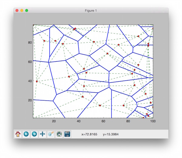
You can execute TinBuild.py, plotting both Voronoi and Delaunay tessellation interactively with the following commandline and options.

python TinBuild.py -v -t -p test.pts

Another test program is TinAlgoTest.py. It generates 100 random points to construct both Voronoi and Delaunay tessellation. Then, it plots the output to the matplotlib window.

• Note: TinAlgo.py only requires the standard Python library. However, if you want to use the plotting function provided by TinAlgoTest.py or TinBuild.py, NumPy and mathplotlib modules are needed.

References

• [Guibas & Stolfi 85] Leonidas Guibas and Jorge Stolfi, Primitives for the Manipulation of General Subdivisions and the Computation of Voronoi Diagrams, ACM Trans. on Graphics, Vol 4. no.2, April 1985, pp 75-123.