artwork by Style of text data transfer to Malevich's Bureau and Room
Deep Learning on Text Data
Large quantity of human communication is composed in the form of text written in natural language. The recent advance in the field of Machine Learning confirms that meaningful knowledge can be extracted effectively. Once the general techniques of natural language processing in combination of machine learning, a wide-range of practical enterprise application can be imagined.
[2024/10/07] We can listen to this article as a Podcast Discussion, which is generated by Google’s Experimental NotebookLM. The AI hosts are both funny and insightful.
images/deep-learning-on-text-data/Podcast_Deep_Learning_on_Text.mp3

Figure. Text data projected onto Van Gogh’s Starry Night painting, as an analogy to the dream of finding patterns out of deceptive chaos.
What we want to learn is how to apply the machine learning technique - Deep Learning to text data. Not surprisingly, the business has abundance of text data, which is usually in the form of unstructured text, that could be emails, comments, or documents that is chaotic in it’s original form. For Machine Learning, finding patterns out of this deceptive chaos automatically is the engineering dream of AI. To tackle this natural language chaos, ML developer has the Natural Language Processing (NLP) techniques to discover patterns. In this article, we shall start with the theoretical knowledge of NLP applied to ML, then we shall practice the techniques on the twitter’s sentiment analysis problem, and apply Deep Learning to model and predict the tweets sentiment.
Sentiment Analysis with Machine Learning
Sentiment Analysis is a pretty interesting problem in the NLP space. Whenever there is an email coming into the customer service inbox, the business wants to be able to identify the customer’s sentiment, and in the case that the customer’s sentiment is negative, we want to send it to the customer service folder for attention; otherwise we want to send it to the happy feedback inbox. One way to solve this problem is to handcraft a complex set of rules and then actually implement a program that will check whether these rules are satisfied. When an email arrived, it would go through an algorithm that will check for the static rules and the output would be a label that says whether this email’s is positive or negative sentiment.
The static rules could be, for example like a check, which looks for specific keywords being present in the email or not. If those keywords were present, then it would send it to the customer service folder. Possibly, this kind of approach is perfectly alright with some business. But given the complexity of natural language and the types of problems, even human expert may find that difficult to express in rules. In such case, if the business happen to have a large amount of historical emails, basically a large body of text already available. In addition, if the patterns or relationships that the business are trying to model dynamically and continuously changing, then using a machine learning approach will be a better option than a rule based approach.
Within a machine learning approach, we would design part of the system where an email is coming in, it goes through a trained model which is checking for the email sentiments, and the model will return an output which says positive or negative. The only difference here is that the rules, which are used to check whether an email is positive or negative sentiment, are dependent on historical emails. So the ML algorithm would basically look at historical emails to derive the rules and it would keep updating the rules as the business accumulates more and more historical emails. The historical emails, which have already been marked as positive and negative sentiment, embedded within them a lot of information which indicate what makes an email as positive or negative sentiment. The ML algorithm is able to look at the historical emails, and infer what those rules are by itself, and use those rules to check against any new email; subsequently, classify it into positive or negative sentiment correctly.
Types of Machine Learning in NLP
There are two approaches that we could take while solving any NLP problem. The rule based approach would involve the programmer either knowing what the rules are or empirically identifying the rules by using data analytics and exploration. In the machine learning approach, the rules will be identified by an ML algorithm. But there is a workflow that needs to be set up first.
Machine learning problems generally fall under a specific set of categories. You would start by identifying which type of problem or which category the problem you are trying to solve falls into. Once the problem’s category has been identified, the data need to be transformed and represented by using numeric attributes. Then, we would apply a standard ML algorithm on those numeric data.
As previously mentioned, machine learning problems generally fall under a broad set of categories. These categories include classification clustering, recommendations, and regression. Since the email sentiment problem that we are trying to solve belongs to classification, we concentrate the investigation on classification clustering.
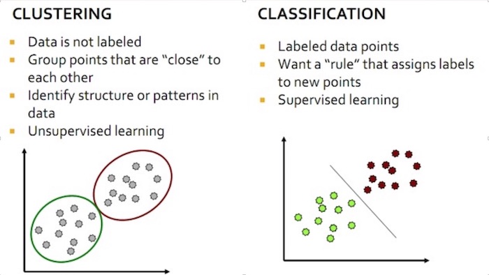
Figure. Showing the key differences between clustering and classification in machine learning.
Classification
Classification is one of the most common type of NLP tasks that happens in machine learning, for example, performing sentiment analysis to classify a piece of text as positive or negative sentiment or classifying a bunch of articles into one of a different set of genres. For instance, an email or a tweet could be the target problem instance. This problem instance needs to be classified into one of a number of categories. We need to assign a category or a label to the problem instance. In the sentiment analysis problem, the labels are positive (numerically as 1) and negative (numerically as 0).
ML algorithms which help to perform classification are known as Classifiers. In order to use a Classifier, there is a prerequisite. The prerequisite is that a set of instances for which the correct category membership is known. If you are performing sentiment analysis, a set of tweets which are already classified as positive or negative. This set of tweets is called training data and it is from this data that the Classifier infers the rules or patterns that actually help to classify a new tweets as positive or negative.
Clustering
Another class of machine learning problems, which are pretty common in NLP is Clustering. For example, a set of articles needs to be identified with the themes or topics according to their content. The articles having some common attributes are identified as relating to each others. The key thing here, as compared to classification, is that the article’s grouping are unknown before we start. So using the clustering algorithm, the large set of articles is clustered into the smaller groups. Once we have the clusters, these groups have some shared attributes and meaning representing particular theme or topic. Clustering is usually used to just explore the data, explore the body of text, and to identify patterns existed within that set.
With these identified patterns as guidance, we can determine what is the best machine learning workflow to be applied.
Mechanics of Machine Learning on Text Data
After the type of problem has been identified, the next step is to identify numeric attributes from the text. The numeric attributes are used to represent each piece of text. Since the ML algorithms only take numeric data as input, the input text needs to be converted into it’s numeric representation. The numeric attributes are called features. There are different methods that the text can be transformed into these numeric attributes.
One example is called term frequency representation, which looks at frequencies of words which occur in the text. Another example is term frequency inverse-document frequency. We’ll look at both of these methods as we go on through the example.
Once the data is read in a numeric form, you can take a standard algorithm and then apply it on the data. The job of the algorithm is to find patterns from historical data. So it takes historical data, which could be a large body of text that you are feeding to the algorithm in the form of numeric attributes, and it will identify rules that quantify relationships between those numeric attributes.
These rules that the ML algorithm identifies, form together as a Model. The Model is simply the representation of the patterns that are identified by the algorithm. It can be something like a mathematical equation or it could be a set of rules which are represented as if-then-else statements. In terms of neural network, it is the set of neuron weights in the network.
- For a classification problem, algorithms like the Naive Bayes, the Support Vector Machines or Deep Learning can be applied.
- Alternatively, for a clustering problem, algorithms like K-means Clustering or Hierarchical Clustering can be chosen.
Twitter Sentiment Analysis
Machine Learning is an extremely useful tool to solve the text data problems. We can apply the essential ML workflow on text data,
- Prepare Data - using tokenization, stopword removal, word sense disambiguation and etc.
- Train Model - using unsupervised clustering, supervised classification ML algorithms.
- Evaluate Model - measuring the model performance to continue improving the model.
Prepare Data
The text data is usually run through a series of preprocessing tasks, to take a large piece of text and then break it down into smaller and meaningful components. The mixture of following tasks are applied depending on the data set requirements,
- Tokenization - breaking down he individual sentences or individual words themselves are the process called tokenization.
- Stopwords - isolating the individual words or tokens in the text, some words that does not add information or meaning to the text, and the others which are just present to add structure or for grammatical purposes. These called stopwords, that could be words like “is” and “the”, the lists of stopwords can be filtered out before further processing of the text.
- N-Gram - identifying what are the most commonly occurring words in the text because these are the most important words in the text and finding groups of words that occur together are the task of n-gram, would extract more meaning out of the text.
- Stemming - extracting only the root of the word, for example ‘closed’ becomes ‘close’ because they have the same meaning, is called stemming.
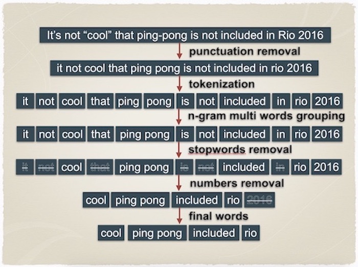
Figure. An example of text pre-processing workflow and the processing results
The techniques to convert textual data into other representations are,
- Disambiguation - identifying the meaning of the word based on the context in which it occurs. The sentence is parsed on identifying which part of speech, whether a word, or a noun, or an adverb, and so on.
- Word2Vec - vectorized word into multi-dimensional space based on their context and meaning within the group of text.
Prepare Tweets Data
The tweets data can be downloaded from The Twitter Sentiment Analysis Dataset.
It’s a csv file that contains 1.6 million rows. Each row has amongst other things, the text of the tweet and the corresponding sentiment.
Each tweet is marked as 1 for positive sentiment and 0 for negative sentiment.
The original downloaded sentiment tweets needs some preprocessing to clean up the csv file.
In particular, the SentimentText column needs to be quoted properly.
The following script will surround the original tweets with quotes, and clean up quotes within the outer quote,
to make the data format consumable by the Pandas’s csv parser to construct the dataframe.
fname = "tweets_download.csv"
with open(fname) as f:
    content = f.readlines()

content = [x.strip().split(',', 3) for x in content]
f.close()

fname = "tweets.csv"
with open(fname, 'w') as f:
    f.write('"ItemID","Sentiment","SentimentSource","SentimentText"\n')
    for x in content[1:]:
        f.write('"' + x[0] + '"')
        f.write(',')
        f.write('"' + x[1] + '"')
        f.write(',')
        f.write('"' + x[2] + '"')
        f.write(',')
        y = x[3].replace('"', '')
        f.write('"' + y + '"')
        f.write('\n')

f.close()
After cleaning up the " quote problems, we can load the tweets from the result tweets.csv into Pandas dataframe.
import pandas as pd

tweets = pd.read_csv("tweets.csv")
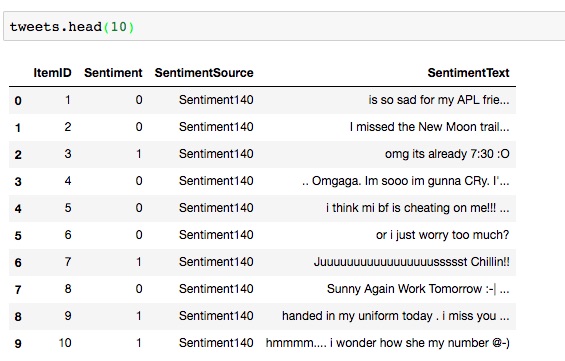
The dataframe tweets can be inspected for deeper insight into the tweet data,
for example, starting with displaying the first 10 rows, and more.
Tweet Text Preprocessing
We want to break each tweet into meaningful words.
The tokenizer_tweet() function, calling tokenizer(), is for the tweet’s tokenization, stopwords and punctuation removal.
The tweet’s specific filtering is isolated in tokenizer_tweet(),
while keeping tokenizer() generic for any text data for potential reuse.
import re
import nltk
from nltk.tokenize import word_tokenize, sent_tokenize
from nltk.corpus import stopwords
from string import punctuation

# list of stopwords like articles, preposition
stop = set(stopwords.words('english'))

def tokenizer(text):
    try:
        tokens_ = [word_tokenize(sent) for sent in sent_tokenize(text)]

        tokens = []
        for token_by_sent in tokens_:
            tokens += token_by_sent

        tokens = list(filter(lambda t: t.lower() not in stop, tokens))
        tokens = list(filter(lambda t: t not in punctuation, tokens))

        filtered_tokens = []
        for token in tokens:
            if re.search('[a-zA-Z]', token):
                filtered_tokens.append(token)

        filtered_tokens = list(map(lambda token: token.lower(), filtered_tokens))

        return filtered_tokens
    except Exception as e:
        print(e)

def tokenizer_tweet(tweet):
    tweet = unicode(tweet.decode('utf-8').lower())
    tokens = tokenizer(tweet)
    tokens = filter(lambda t: not t.startswith('@'), tokens)
    tokens = filter(lambda t: not t.startswith('#'), tokens)
    tokens = filter(lambda t: not t.startswith('http'), tokens)
    return tokens
Discover Important Words
The exploration never stops after the text pre-processing.
With the tokenized words, we must proceed to answer the question of what are the important words for the problem domain? First, we present a typical text analytic step using tf-idf (term frequency-inverse document frequency) to find the important words. The effort to understand tf-idf concept is still important for the text analysis in general; however, we shall show the reason why tf-idf words do not fit in the sentiment analysis.
Then, we show that the simple word counting is sufficient for identifying the tweet important words.
(1) By tf-idf
To analyze a corpus of text, we like to know what are the important words. tf-idf stands for term frequency-inverse document frequency. It’s a numerical statistic intended to reflect how important a word is to a document or a corpus (i.e. a collection of documents).
To relate to this post, words correspond to tokens and documents correspond to descriptions. A corpus is therefore a collection of descriptions.
The tf-idf of a term t in a document d is proportional to the number of times the word t appears in the document d but is also offset by the frequency of the term t in the collection of the documents of the corpus. This helps adjusting the fact that some words appear more frequently in general and don’t especially carry a meaning.
tf-idf acts therefore as a weighting scheme to extract relevant words in a document.
\[tfidf(t,d) = tf(t,d) . idf(t)\]\(tf(t,d)\) is the term frequency of t in the document d (i.e. how many times the token t appears in the description d)
\(idf(t)\) is the inverse document frequency of the term t. it’s computed by this formula:
\[idf(t) = log(1 + \frac{1 + n_d}{1 + df(d,t)})\]- \(n_d\) is the number of documents
- \(df(d,t)\) is the number of documents (or descriptions) containing the term t
Computing the tfidf matrix is done using the TfidfVectorizer() method from scikit-learn. Let’s see how to do this:
from sklearn.feature_extraction.text import TfidfVectorizer

# min_df is minimum number of documents that contain a term t
# max_features is maximum number of unique tokens (across documents) that we'd consider
# TfidfVectorizer preprocesses the descriptions using the tokenizer we defined above
vectorizer = TfidfVectorizer(min_df=10, max_features=10000, tokenizer=tokenizer, ngram_range=(1, 2))
vz = vectorizer.fit_transform(list(tweets['SentimentText']))
vz is a tfidf matrix.
- it’s number of rows is the total number of documents (descriptions)
- it’s number of columns is the total number of unique terms (tokens) across the documents (descriptions)
\(x_{dt} = tfidf(t,d)\) where \(x_{dt}\) is the element at the index (d,t) in the matrix.
Let’s create a dictionary mapping the tokens to their tfidf values
tfidf = dict(zip(vectorizer.get_feature_names(), vectorizer.idf_))
tfidf = pd.DataFrame(columns=['tfidf']).from_dict(dict(tfidf), orient='index')
tfidf.columns = ['tfidf']
We can visualize the distribution of the tfidf scores by histogram
tfidf.tfidf.hist(bins=50, figsize=(15,7))
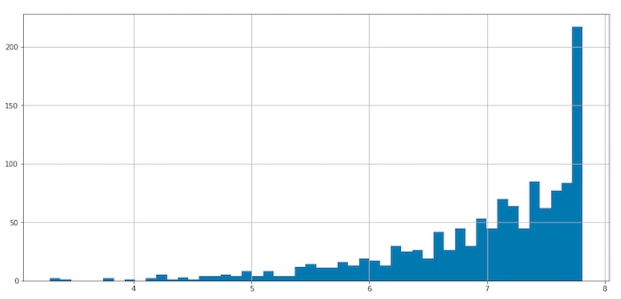
Figure. tf-idf scores historgram, high tf-idf score means more discriminated word; otherwise low tf-idf means less discriminated word.
We tried to see the tf-idf score for some of the obvious sentimental words. Not too surprising, these words are not very discriminated because they are used very often within the corpus.
tfidf.loc[['sorry','happy','sad']]
| tfidf | |
|---|---|
| sorry | 5.710631 |
| happy | 5.092447 |
| sad | 4.721503 |
Some of the top discriminated words can be found by,
tfidf.sort_values(by=['tfidf'], ascending=False).head(3)
| tfidf | |
|---|---|
| window | 7.812545 |
| maths | 7.812545 |
| grandma | 7.812545 |
This tell us that {window, maths, grandma} are the words seldom used in the tweets. If a tweet contains these words, that shows a lot more special than the other words. But to the sentiment analysis, it is not trying to locate highly discriminated words; instead, the words are commonly used and recognized as sentimental should be ranked higher.
(2) By Counting
Failing to use the more sophisticated and popular tf-idf technique to discover the important words, the mundane technique of word counting is tested.
import collections

counter = collections.Counter()
maxlen = 0
for index, tweet in tweets.iterrows():
    try:
        words = [x.lower() for x in tokenizer_tweet(tweet["SentimentText"])]
        if len(words) > maxlen:
            maxlen = len(words)
        for word in words:
            counter[word] += 1
    except:
        pass
Surprisely, just by inspecting the top 10 most commonly used words in the tweets, we discovered that the sentimental words are among the most commonly used words.
counter.most_common(10)

[(u"'s", 179509),
 (u"n't", 173837),
 (u"'m", 130868),
 (u'good', 88554),
 (u'day', 82165),
 (u'get', 81338),
 (u'like', 77753),
 (u'go', 72547),
 (u'quot', 71387),
 (u'got', 69689)]
We resort to settle with the simple counting technique to build our vocabulary for machine learning.
Our vocabulary will be the top common words, with VOCAB_SIZE (=5000) words from the tweets.
As a side note, we reserved the word index 0 to unknown _UNK_, for any other words that does not appear in our vocabulary,
we shall assign those words as unknown. Consequently, the deep learning will treat those words as the anonymous _UNK_.
VOCAB_SIZE = 5000

word2index = collections.defaultdict(int)
for wid, word in enumerate(counter.most_common(VOCAB_SIZE)):
    word2index[word[0]] = wid + 1
vocab_sz = len(word2index) + 1
index2word = {v:k for k, v in word2index.items()}
index2word[0] = "_UNK_"
Converting Word to Numeric Representation by word2vec
Only invented recently, the advanced technique of word2vec is used to convert word into numeric representation. word2vec is a group of Deep Learning models developed by Google with the aim of capturing the context of words while at the same time proposing a very efficient way of preprocessing raw text data. This model takes as input a large corpus of documents like tweets or news articles and generates a vector space of typically several hundred dimensions. Each word in the corpus is being assigned a unique vector in the vector space.
For example, as shown in the following figure from Tomas Mikolov’s presentation at NIPS 2013, vectors connecting words that have similar meanings but opposite genders are approximately parallel in the reduced 2D space, and we can often get very intuitive results by doing arithmetic with the word vectors. The presentation provides many other examples.
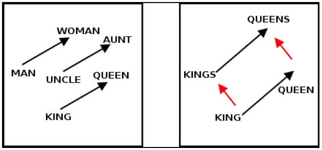
Figure. (left) Illustrates word2vec vectors that has close proximity to similar meaning words. (right) Illustrates word2vec vectors detect multiple features on different levels of abstractions.
For our purpose, download the word2vec GoogleNews Vectors as the starting point, this data has been pre-trained with Google News corpus (3 billion words) word vector model (containing 3 million 300-dimension English word vectors).
After downloading the word2vec data, we can load it with gensim.models.KeyedVectors.
from gensim.models import KeyedVectors

WORD2VEC_MODEL = "data/GoogleNews-vectors-negative300.bin.gz"
word2vec = KeyedVectors.load_word2vec_format(WORD2VEC_MODEL, binary=True)
To gain some intuitive idea about word2vec, for example, the word man vectorized as a 300 dimension point as shown.
print word2vec['man']

[ 0.32617188  0.13085938  0.03466797 -0.08300781  0.08984375 -0.04125977
 -0.19824219  0.00689697  0.14355469  0.0019455   0.02880859 -0.25
 -0.08398438 -0.15136719 -0.10205078  0.04077148 -0.09765625  0.05932617
  0.02978516 -0.10058594 -0.13085938  0.001297    0.02612305 -0.27148438
  0.06396484 -0.19140625 -0.078125    0.25976562  0.375      -0.04541016
  ...
  0.07177734  0.13964844  0.15527344 -0.03125    -0.20214844 -0.12988281
 -0.10058594 -0.06396484 -0.08349609 -0.30273438 -0.08007812  0.02099609 ]
The powerful concept behind word2vec is that word vectors that are close to each other in the vector space represent words that are not only of the same meaning but of the same context as well. When we are looking for the most similar words, word2vec yeilds the following result.
word2vec.most_similar('man')

[(u'woman', 0.7664012908935547),
 (u'boy', 0.6824870705604553),
 (u'teenager', 0.6586930751800537),
 (u'teenage_girl', 0.6147903800010681),
 (u'girl', 0.5921714901924133),
 (u'suspected_purse_snatcher', 0.571636438369751),
 (u'robber', 0.5585119128227234),
 (u'Robbery_suspect', 0.5584409236907959),
 (u'teen_ager', 0.5549196600914001),
 (u'men', 0.5489763021469116)]
What we find interesting about the vector representation of words is that it automatically embeds several features that normally have to be handcrafted. Since word2vec relies on deep neural network to detect patterns, we can also rely on word2vec to detect multiple features on different levels of abstractions.
notice the funny thing about “man” is most similar to “robber” and “Robbery_suspect”. This must be influenced by the set of news sources where the word2vec is constructed.
For each word index, the corresponding word2vec vector is assigned into embbeding_weights matrix.
This matrix will be used for converting word into word2vec representation later.
import numpy as np

embedding_weights = np.zeros((vocab_sz, EMBED_SIZE))
for word, index in word2index.items():
    try:
        embedding_weights[index, :] = word2vec[word]
    except KeyError:
        pass
For example, if the word man is in vocabulary word2index['man']=123,
then the vectorized word man is represented by embbedding_weights[123].
Train Model with Keras
To keep focus, we shall not divert to explain keras deep learning framework. Interested reader should consult the book by Antonio Gulli & Sujit Pal, Deep Learning with Keras.
Prepare Data Set
Even more data preparation! we need to reformat the tweets into the suitable vector format for the keras layers to consume.
The following vectors are constructed,
Xis the input tweet word vectorsYis the sentiment label, 0 is negative and 1 is positive sentimentTextis the tweet “SentimentText” (we shall use this vector for displaying the tweet, along with the prediction results later)
from keras.preprocessing.sequence import pad_sequences
from keras.utils import np_utils

ts = []
xs = []
ys = []
for index, tweet in tweets.iterrows():
    try:
        ts.append(tweet["SentimentText"])
        ys.append(tweet["Sentiment"])
        words = [x.lower() for x in tokenizer_tweet(tweet["SentimentText"])]
        wids = [word2index[word] for word in words]
        xs.append(wids)
    except:
        print tweet

Text = ts
X = pad_sequences(xs, maxlen=maxlen)
Y = np_utils.to_categorical(ys)
Split Data Set
The usual data splitting recommendation is 70/30 of the training/testing data set.
We use the sklearn.model_selection utility train_test_split() function to randomize the splitting.
Noticing the parameter test_size=0.3, means 30% will be allocated to testing data set.
We set the initial random_state=42 for reproducible of the data set, to support multiple runs with the same splitting sequence.
from sklearn.model_selection import train_test_split

Xtrain, Xtest, Ytrain, Ytest = train_test_split(X, Y,
                                                test_size=0.3,
                                                random_state=42)
# perform the exactly same splitting for the corresponding Text vector
Xtrain, Xtest, Ttrain, Ttest = train_test_split(X, Text,
                                                test_size=0.3,
                                                random_state=42)
Deep Learning
We define and train the Deep Learning neural network with keras.
(1) Define Deep Neural Network
We initialize the weights of the embedding layer with the embedding_weights matrix
that we built in the previous section.
The model is compiled with the binary-crossentropy loss function (because we only have 2 classes) and the adam
optimizer.
from keras.layers.core import Dense, Dropout
from keras.layers.convolutional import Conv1D
from keras.layers.embeddings import Embedding
from keras.layers.pooling import GlobalMaxPooling1D
from keras.models import Sequential
from keras import regularizers

EMBED_SIZE = 300
NUM_FILTERS = 128
NUM_WORDS = 3

model = Sequential()
model.add(Embedding(vocab_sz, EMBED_SIZE, input_length=maxlen,
                    weights=[embedding_weights],
                    embeddings_regularizer=regularizers.l2(0.01),
                    trainable=True))
model.add(Dropout(0.5))
model.add(Conv1D(filters=NUM_FILTERS, kernel_size=NUM_WORDS,
                 activation="relu"))
model.add(Dropout(0.5))
model.add(GlobalMaxPooling1D())
model.add(Dense(sentiment_len, activation="sigmoid"))

model.compile(optimizer="adam", loss="binary_crossentropy",
              metrics=["accuracy"])
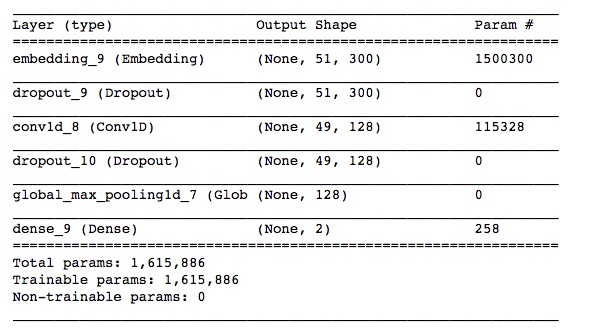
The Deep Learning network is summarized by the summary() function.
model.summary()
(2) Train Deep Neural Network
We shall invoke the network training by model.fit(),
and train the network with batch size 16 and for 20 epochs, then evaluate the trained model.
BATCH_SIZE = 16
NUM_EPOCHS = 20
history = model.fit(Xtrain, Ytrain, batch_size=BATCH_SIZE,
                    epochs=NUM_EPOCHS,
                    validation_data=(Xtest, Ytest))
After 20 epoches of training, the accuracy is converged to ~72%.
Train on 1104929 samples, validate on 473542 samples
Epoch 1/20
1104929/1104929 [==============================] - 1966s 2ms/step - loss: 1.4675 - acc: 0.7124 - val_loss: 0.8175 - val_acc: 0.7212
...
Epoch 20/20
1104929/1104929 [==============================] - 1941s 2ms/step - loss: 0.8374 - acc: 0.7174 - val_loss: 0.8260 - val_acc: 0.7221
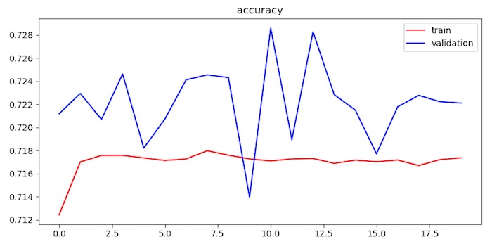
Figure. The chart show the training accuracy and validation accuracy. The training accuracy has converged quickly.
(3) Evalute Trained Model
The model gives us an accuracy of 72.2% on the test set after 20 epochs of training.
score = model.evaluate(Xtest, Ytest, verbose=1)
print("Test score: {:.3f}, accuracy: {:.3f}".format(score[0], score[1]))

473542/473542 [==============================] - 85s 180us/step
Test score: 0.826, accuracy: 0.722
Evaluate Model for Further Improvements
The model prediction accuracy is good but not super.
Since keras can return the prediction vector for each classification,
in our case there are 2 classes (0 negative and 1 positive sentiment),
we can perform further analysis on comparing the actual vs prediction results;
hopefully, the analysis can reveal clues to improve the model.
Ypredict = model.predict(Xtest, batch_size=32, verbose=1)
print Ypredict[:5]
We can see the prediction probability vector, for each row (a tweet) and column (probability for each class). The total probabilities for each row should be 1.
array([[ 0.25863048,  0.74136955],
       [ 0.69782579,  0.30217424],
       [ 0.20225964,  0.79774034],
       [ 0.16227043,  0.83772963],
       [ 0.74099219,  0.25900784]], dtype=float32)
(0) Find the Corresponding Actual and Predict Sentiment
This is a data preparation to construct vectors to support analysis.
We can collect the actual_sentiment label and the predict_sentiment label for each tweet.
For the sentiment classification, selecting the index with the highest probability, which will yeild the predicted label.
actual_sentiment_idx = np.argmax(Ytest, axis=1)
actual_sentiment = [id2sentiment[k] for k in actual_sentiment_idx]
predict_sentiment_idx = np.argmax(Ypredict, axis=1)
predict_sentiment = [id2sentiment[k] for k in predict_sentiment_idx]
predict_probs = np.array([Ypredict[k][predict_sentiment_idx[k]] for k in np.arange(len(predict_sentiment_idx))])
(1) Review Correct Predicted Labels at Random
We can review the correct predicted labels at random, and print out with the tweet.
correct = np.where(predict_sentiment_idx==actual_sentiment_idx)[0]
print("Found %d correct labels of %d" % (len(correct), len(predict_sentiment_idx)))
idx = permutation(correct)[:5]
for i in idx:
    print("[%d] predict '%s' -> actual '%s': '%s'" %(i, predict_sentiment[i], actual_sentiment[i], Ttest[i]))
The results shows the prediction along with the tweets.
Found 341950 correct labels of 473542
[61746] predict '0' -> actual '0': 'I'm off to work, be back around 11pm  I hate long work days'
[25913] predict '1' -> actual '1': 'Jus woke up!!!!!!! Crazy night'
[85662] predict '1' -> actual '1': '"Kids" on repeat. Absolutely amazing! So fatigued right now but we're leaving 4 Norway today'
[202167] predict '0' -> actual '0': '@RoxygirlSLB nah didn't say that but she probably would have one! Hehe I want a black one, but they don't do them in UK'
[165979] predict '1' -> actual '1': 'Aww! Zack & Vanessa are so cute together.'
(2) Review Incorrect Predicted Labels at Random
We can review the incorrect predicted labels at random, and print out with the tweet.
incorrect = np.where(predict_sentiment_idx!=actual_sentiment_idx)[0]
print("Found %d incorrect labels of %d" % (len(incorrect), len(predict_sentiment_idx)))
idx = permutation(incorrect)[:5]
for i in idx:
    print("[%d] predict '%s' -> actual '%s': '%s'" %(i, predict_sentiment[i], actual_sentiment[i], Ttest[i]))
The results shows the incorrect prediction along with the tweets. The failure shows the subtlety of the tweets, for example ‘Oh happy day. Not’, the network incorrectly predicted positive sentiment. The distant word ‘Not’ seems to be negation factor to the ‘happy’ word in the tweet.
Found 131592 incorrect labels of 473542
[241731] predict '0' -> actual '1': '@astynes Yr norty!  When we try copy a big disc like that we have to forfeit some of the quality 2 fit it on. It's a gr8 disc 2 watch tho!'
[235609] predict '1' -> actual '0': 'Oh happy day. Not'
[220989] predict '0' -> actual '1': 'My first day in Twitter It will be interesting I think So do you want to see my hometown?  http://www.admkrsk.ru/doc.asp?id=12'
[315661] predict '0' -> actual '1': 'Working on transfer papers, then lunch with Luke.'
[340588] predict '1' -> actual '0': 'business business business  bye bye awards
(3) Review the Most Confident Predicted Labels that are Correct
We can review the most confident prediected labels that are correct, for each class.
for sent in range(0,sentiment_len):
    correct_sent = np.where((predict_sentiment_idx==sent) & (predict_sentiment_idx==actual_sentiment_idx))[0]
    print("Found %d confident correct %d:'%s' category" % (len(correct_sent), sent, id2sentiment[sent]))
    if (len(correct_sent) > 0):
        most_correct_sent = np.argsort(predict_probs[correct_sent])[::-1][:4]
        for k in most_correct_sent:
            print("[%d] predict '%s' with %.3f confidence: '%s'" %(correct_sent[k], predict_sentiment[correct_sent[k]], predict_probs[correct_sent[k]], Ttest[k]))
The results of the most confident prediction along with the tweets.
Found 185735 confident correct 1:'1' category
[57266] predict '1' with 0.974 confidence: '@n8moses What fun! Hope you brought yummies for them'
[443611] predict '1' with 0.973 confidence: 'can't say I've had a Friday go this bad this fast before!'
[100613] predict '1' with 0.973 confidence: 'OMG my dog just attacked the baby possum  we think its ok but not positive.... -fingers crossed-'
[253526] predict '1' with 0.969 confidence: 'E3 looks awsome this year i missed microsofts keynote though  damn!'
(4) Review the Most Confident Predicted Labels that are Incorrect
We can review the most confident prediected labels that are incorrect, for each class.
for sent in range(0,sentiment_len):
    incorrect_sent = np.where((predict_sentiment_idx==sent) & (predict_sentiment_idx!=actual_sentiment_idx))[0]
    print("Found %d confident incorrect %d:'%s' category" % (len(incorrect_sent), sent, id2sentiment[sent]))
    if (len(incorrect_sent) > 0):
        most_incorrect_sent = np.argsort(predict_probs[incorrect_sent])[::-1][:4]
        for k in most_incorrect_sent:
            print("[%d] predict '%s' but actual '%s' with %.3f confidence: '%s'" %(incorrect_sent[k], predict_sentiment[incorrect_sent[k]], actual_sentiment[incorrect_sent[k]], predict_probs[incorrect_sent[k]], Ttest[k]))
The results of the most confident incorrect prediction along with the tweets.
Found 80332 confident incorrect 0:'0' category
[398966] predict '1' but actual '0' with 0.962 confidence: 'I cnt bel eive im saying this an ino i sudnt but i kinda love lois'
[425603] predict '1' but actual '0' with 0.961 confidence: 'was almost in a wreck and mcdonalds was too crowded for me to stop, so now i'm shaking AND hungry'
[340460] predict '1' but actual '0' with 0.961 confidence: '#phpkonferenca anže is beeing funny'
[87609] predict '1' but actual '0' with 0.958 confidence: 'Also my niece has better brand names than me. Girl is rockin pink baby phat blankets'
(5) Review by the Confusion Matrix
Perhaps the most common way to analyze the result of a classification model is to use a confusion matrix.
scikit-learn has a convenient confusion_matrix() function for this purpose:
from sklearn.metrics import confusion_matrix

cm = confusion_matrix(actual_sentiment_idx, predict_sentiment_idx)
We can just print out the confusion matrix, or we can show a graphical view (which is mainly useful for a larger number of categories).
import matplotlib.pyplot as plt

def plot_confusion_matrix(cm, classes, normalize=False, title='Confusion matrix', cmap=plt.cm.Blues):
    """
    This function prints and plots the confusion matrix.
    Normalization can be applied by setting `normalize=True`.
    (This function is copied from the scikit docs.)
    """
    plt.figure(figsize=(8, 8), dpi=100)
    plt.imshow(cm, interpolation='nearest', cmap=cmap)
    plt.title(title)
    plt.colorbar()
    tick_marks = np.arange(len(classes))
    plt.xticks(tick_marks, classes, rotation=45)
    plt.yticks(tick_marks, classes)

    if normalize:
        cm = cm.astype('float') / cm.sum(axis=1)[:, np.newaxis]
    print(cm)
    thresh = cm.max() / 2.

    plt.tight_layout()
    plt.ylabel('True label')
    plt.xlabel('Predicted label')
Calling plot_confusion_matrix() to plot,
plot_confusion_matrix(cm, [id2sentiment[i] for i in range(0,sentiment_len)])
The confusion matrix looks like,
[[156215  80332]
 [ 51260 185735]]
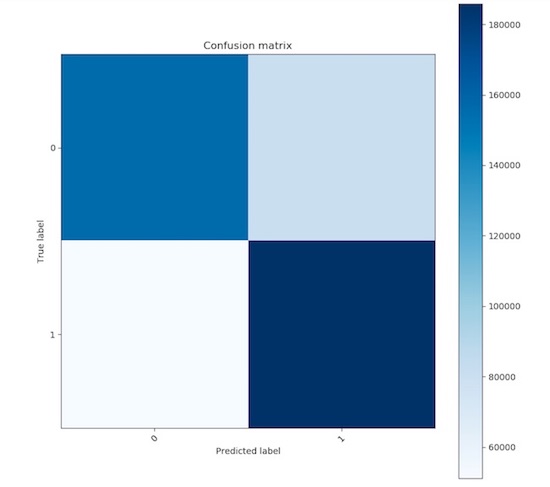
The model tends to incorrectly predict negative sentiment as positive sentiment more often.
Further Improvements
For further improvements, the analysis definitely gives some clues on how to enhance the model,
- increase the vocabulary size
- increase weights for those sentimental words
- ignore unknown words that is not in English dictionary
- improve the network with more advanced deep learning layers, e.g. RNN, for bigger context
References
- Antonio Gulli & Sujit Pal, Deep Learning with Keras, Packt Publishing, Apr 2017, ISBN: 978-1-78712-842-2
- Ahmed Besbes, Sentiment Analysis on Twitter using word2vec and keras, Apr 2017.
- Ahmed Besbes, *How to Mine Newsfeed Data and Extract Interactive Insight in Python, Apr 2018.
- T. Mikolov, I. Sutskever, K. Chen, G. S. Corrado, J. Dean, Q. Le, and T. Strohmann, Learning Representations of Text using Neural Networks, NIPS 2013
Hope you enjoy the machine learning adventure on text data as much as we do!